Classification and regression

This chapter is designed to get you started with using neural networks to solve real problems. You'll consolidate the knowledge you gained from chapters 2 and 3, and you'll apply what you've learned to three new tasks covering the three most common use cases of neural networks — binary classification, categorical classification, and scalar regression:

• Classifying movie reviews as positive or negative (binary classification)
• Classifying news wires by topic (categorical classification)
• Estimating the price of a house, given real estate data (scalar regression)

These examples will be your first contact with end-to-end machine learning workflows: you'll get introduced to data preprocessing, basic model architecture principles, and model evaluation.

By the end of this chapter, you'll be able to use neural networks to handle simple classification and regression tasks over vector data. You'll then be ready to start building a more principled, theory-driven understanding of machine learning in chapter 5.

Classifying movie reviews: A binary classification example

Two-class classification, or binary classification, is one of the most common kinds of machine learning problem. In this example, you'll learn to classify movie reviews as positive or negative, based on the text content of the reviews.

The IMDb dataset

You'll work with the IMDb dataset: a set of 50,000 highly polarized reviews from the Internet Movie Database. They're split into 25,000 reviews for training and 25,000 reviews for testing, each set consisting of 50% negative and 50% positive reviews.

Just like the MNIST dataset, the IMDb dataset comes packaged with Keras. It has already been preprocessed: the reviews (sequences of words) have been turned into sequences of integers, where each integer stands for a specific word in a dictionary. This enables us to focus on model building, training, and evaluation. In chapter 14, you'll learn how to process raw text input from scratch.

The following code will load the dataset (when you run it the first time, about 80 MB of data will be downloaded to your machine).

from keras.datasets import imdb

(train_data, train_labels), (test_data, test_labels) = imdb.load_data(
    num_words=10000
)

The argument num_words=10000 means you'll only keep the top 10,000 most frequently occurring words in the training data. Rare words will be discarded. This allows you to work with vector data of manageable size. If we didn't set this limit, we'd be working with 88,585 unique words in the training data, which is unnecessarily large. Many of these words only occur in a single sample, and thus can't be meaningfully used for classification.

The variables train_data and test_data are NumPy arrays of reviews; each review is a list of word indices (encoding a sequence of words). train_labels and test_labels are NumPy arrays of 0s and 1s, where 0 stands for negative and 1 stands for positive:

>>> train_data[0]
[1, 14, 22, 16, ... 178, 32]
>>> train_labels[0]
1

Because you're restricting yourself to the top 10,000 most frequent words, no word index will exceed 10,000:

>>> max([max(sequence) for sequence in train_data])
9999

For kicks, let's quickly decode one of these reviews back to English words.

# word_index is a dictionary mapping words to an integer index.
word_index = imdb.get_word_index()
# Reverses it, mapping integer indices to words
reverse_word_index = dict([(value, key) for (key, value) in word_index.items()])
# Decodes the review. Note that the indices are offset by 3 because 0,
# 1, and 2 are reserved indices for "padding," "start of sequence," and
# "unknown."
decoded_review = " ".join(
    [reverse_word_index.get(i - 3, "?") for i in train_data[0]]
)

Let's take a look at what we got:

>>> decoded_review[:100]
? this film was just brilliant casting location scenery story direction everyone

Note that the leading ? corresponds to a start token that has been prefixed to each review.

Preparing the data

You can't directly feed lists of integers into a neural network. They have all different lengths, while a neural network expects to process contiguous batches of data. You have to turn your lists into tensors. There are two ways to do that:

• Pad your lists so that they all have the same length, then turn them into an integer tensor of shape (samples, max_length), and start your model with a layer capable of handling such integer tensors (the Embedding layer, which we'll cover in detail later in the book).

• Multi-hot encode your lists to turn them into vectors of 0s and 1s reflecting the presence or absence of all possible words. This would mean, for instance, turning the sequence [8, 5] into a 10,000-dimensional vector that would be all 0s except for indices 5 and 8, which would be 1s.

Let's go with the latter solution to vectorize the data. When done manually, the process looks like the following.

import numpy as np

def multi_hot_encode(sequences, num_classes):
    # Creates an all-zero matrix of shape (len(sequences), num_classes)
    results = np.zeros((len(sequences), num_classes))
    for i, sequence in enumerate(sequences):
        # Sets specific indices of results[i] to 1s
        results[i][sequence] = 1.0
    return results

# Vectorized training data
x_train = multi_hot_encode(train_data, num_classes=10000)
# Vectorized test data
x_test = multi_hot_encode(test_data, num_classes=10000)

Here's what the samples look like now:

>>> x_train[0]
array([ 0.,  1.,  1., ...,  0.,  0.,  0.])

In addition to vectorizing the input sequences, you should also vectorize their labels, which is straightforward. Our labels are already NumPy arrays, so just convert the type from ints to floats:

y_train = train_labels.astype("float32")
y_test = test_labels.astype("float32")

Now the data is ready to be fed into a neural network.

Building your model

The input data is vectors, and the labels are scalars (1s and 0s): this is one of the simplest problem setups you'll ever encounter. A type of model that performs well on such a problem is a plain stack of densely connected (Dense) layers with relu activations.

There are two key architecture decisions to be made about such a stack of Dense layers:

• How many layers to use
• How many units to choose for each layer

In chapter 5, you'll learn formal principles to guide you in making these choices. For the time being, you'll have to trust us with the following architecture choice:

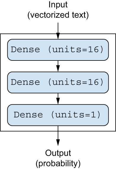
• Two intermediate layers with 16 units each
• A third layer that will output the scalar prediction regarding the sentiment of the current review

Figure 4.1 shows what the model looks like. Here's the Keras implementation, similar to the MNIST example you saw previously.

import keras
from keras import layers

model = keras.Sequential(
    [
        layers.Dense(16, activation="relu"),
        layers.Dense(16, activation="relu"),
        layers.Dense(1, activation="sigmoid"),
    ]
)

The first argument being passed to each Dense layer is the number of units in the layer: the dimensionality of representation space of the layer. You remember from chapters 2 and 3 that each such Dense layer with a relu activation implements the following chain of tensor operations:

output = relu(dot(input, W) + b)

Having 16 units means the weight matrix W will have shape (input_dimension, 16): the dot product with W will project the input data onto a 16-dimensional representation space (and then you'll add the bias vector b and apply the relu operation). You can intuitively understand the dimensionality of your representation space as "how much freedom you're allowing the model to have when learning internal representations." Having more units (a higher-dimensional representation space) allows your model to learn more complex representations, but it makes the model more computationally expensive and may lead to learning unwanted patterns (patterns that will improve performance on the training data but not on the test data).

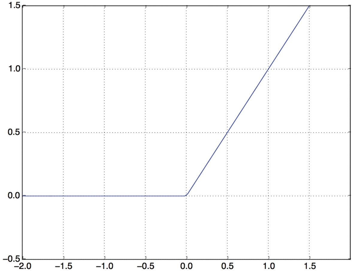
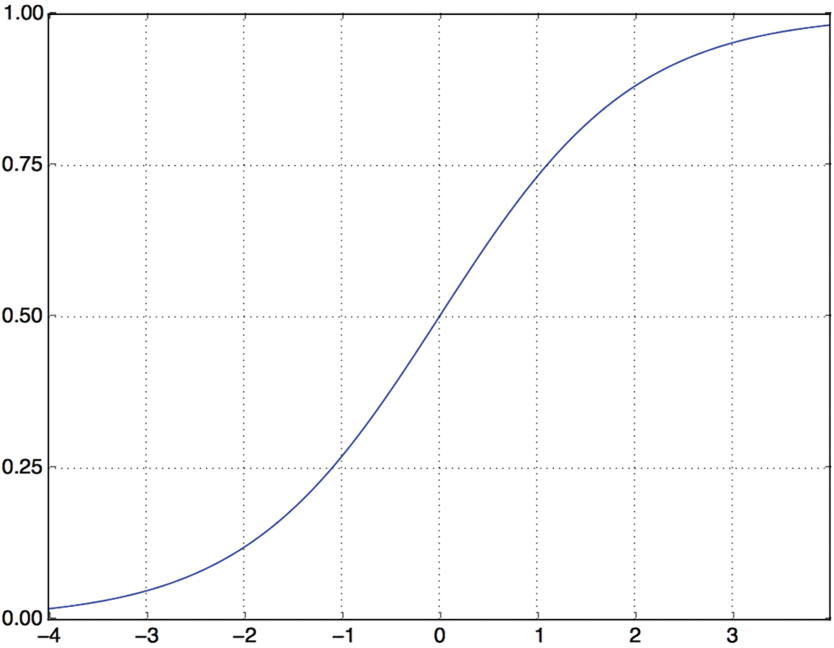
The intermediate layers use relu as their activation function, and the final layer uses a sigmoid activation to output a probability (a score between 0 and 1, indicating how likely the review is to be positive). A relu (rectified linear unit) is a function meant to zero-out negative values (see figure 4.2), whereas a sigmoid "squashes" arbitrary values into the [0, 1] interval (see figure 4.3), outputting something that can be interpreted as a probability.

Finally, you need to choose a loss function and an optimizer. Because you're facing a binary classification problem and the output of your model is a probability (you end your model with a single-unit layer with a sigmoid activation), it's best to use the binary_crossentropy loss. It isn't the only viable choice: you could use, for instance, mean_squared_error. But crossentropy is usually the best choice when you're dealing with models that output probabilities. Crossentropy is a quantity from the field of Information Theory that measures the distance between probability distributions or, in this case, between the ground-truth distribution and your predictions.

As for the choice of the optimizer, we'll go with adam, which is usually a good default choice for virtually any problem.

Here's the step where you configure the model with the adam optimizer and the binary_crossentropy loss function. Note that you'll also monitor accuracy during training.

model.compile(
    optimizer="adam",
    loss="binary_crossentropy",
    metrics=["accuracy"],
)

Validating your approach

As you learned in chapter 3, a deep learning model should never be evaluated on its training data — it's standard practice to use a "validation set" to monitor the accuracy of the model during training. Here, you'll create a validation set by setting apart 10,000 samples from the original training data.

You might ask, why not simply use the test data to evaluate the model? That seems like it would be easier. The reason is that you're going to want to use the results you get on the validation set to inform your next choices to improve training — for instance, your choice of what model size to use or how many epochs to train for. When you start doing this, your validation scores stop being an accurate reflection of the performance of the model on brand-new data, since the model has been deliberately modified to perform better on the validation data. It's good to keep around a set of never-seen-before samples that you can use to perform the final evaluation round in a completely unbiased way, and that's exactly what the test set is. We'll talk more about this in the next chapter.

x_val = x_train[:10000]
partial_x_train = x_train[10000:]
y_val = y_train[:10000]
partial_y_train = y_train[10000:]

You'll now train the model for 20 epochs (20 iterations over all samples in the training data), in mini-batches of 512 samples. At the same time, you'll monitor loss and accuracy on the 10,000 samples that you set apart. You do so by passing the validation data as the validation_data argument to model.fit().

history = model.fit(
    partial_x_train,
    partial_y_train,
    epochs=20,
    batch_size=512,
    validation_data=(x_val, y_val),
)

On CPU, this will take less than 2 seconds per epoch — training is over in 20 seconds. At the end of every epoch, there is a slight pause as the model computes its loss and accuracy on the 10,000 samples of the validation data.

Note that the call to model.fit() returns a History object, as you've seen in chapter 3. This object has a member history, which is a dictionary containing data about everything that happened during training. Let's look at it:

>>> history_dict = history.history
>>> history_dict.keys()
dict_keys(["accuracy", "loss", "val_accuracy", "val_loss"])

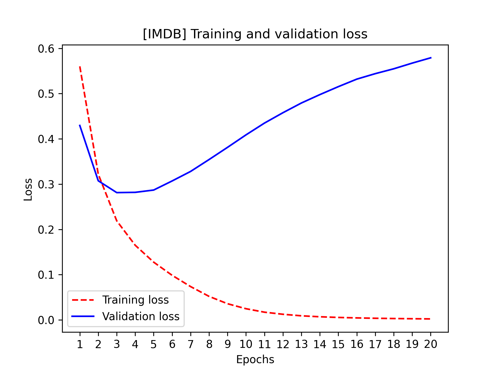
The dictionary contains four entries: one per metric that was being monitored during training and during validation. In the following two listings, let's use Matplotlib to plot the training and validation loss side by side (see figure 4.4), as well as the training and validation accuracy (see figure 4.5). Note that your own results may vary slightly due to a different random initialization of your model.

import matplotlib.pyplot as plt

history_dict = history.history
loss_values = history_dict["loss"]
val_loss_values = history_dict["val_loss"]
epochs = range(1, len(loss_values) + 1)
# "r--" is for "dashed red line."
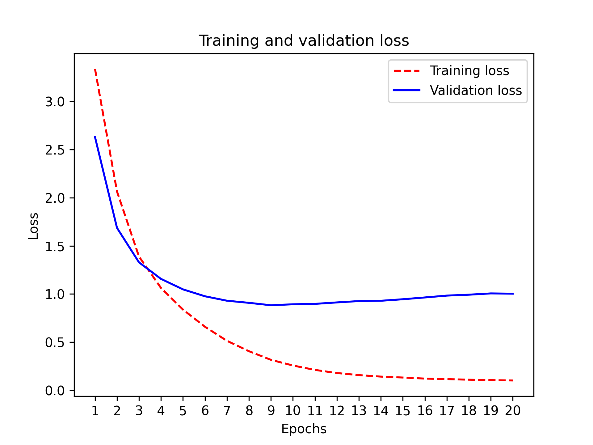
plt.plot(epochs, loss_values, "r--", label="Training loss")
# "b" is for "solid blue line."
plt.plot(epochs, val_loss_values, "b", label="Validation loss")
plt.title("[IMDB] Training and validation loss")
plt.xlabel("Epochs")
plt.xticks(epochs)
plt.ylabel("Loss")
plt.legend()
plt.show()

# Clears the figure
plt.clf()
acc = history_dict["accuracy"]
val_acc = history_dict["val_accuracy"]
plt.plot(epochs, acc, "r--", label="Training acc")
plt.plot(epochs, val_acc, "b", label="Validation acc")
plt.title("[IMDB] Training and validation accuracy")
plt.xlabel("Epochs")
plt.xticks(epochs)
plt.ylabel("Accuracy")
plt.legend()
plt.show()

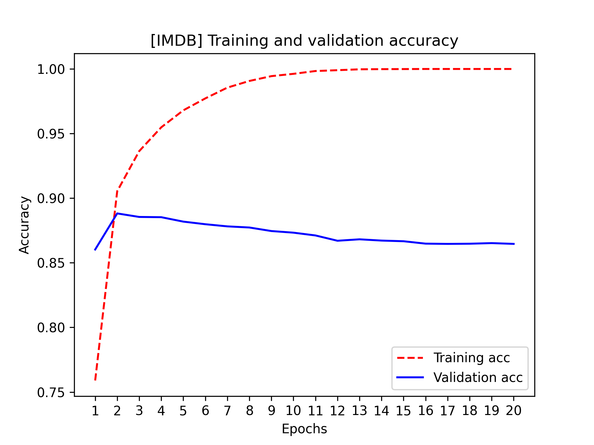
As you can see, the training loss decreases with every epoch, and the training accuracy increases with every epoch. That's what you would expect when running gradient-descent optimization — the quantity you're trying to minimize should be less with every iteration. But that isn't the case for the validation loss and accuracy: they seem to peak at the fourth epoch. This is an example of what we warned against earlier: a model that performs better on the training data isn't necessarily a model that will do better on data it has never seen before. In precise terms, what you're seeing is overfitting: after the fourth epoch, you're over-optimizing on the training data, and you end up learning representations that are specific to the training data and don't generalize to data outside of the training set.

In this case, to prevent overfitting, you could stop training after four epochs. In general, you can use a range of techniques to mitigate overfitting, which we'll cover in chapter 5.

Let's train a new model from scratch for four epochs and then evaluate it on the test data.

model = keras.Sequential(
    [
        layers.Dense(16, activation="relu"),
        layers.Dense(16, activation="relu"),
        layers.Dense(1, activation="sigmoid"),
    ]
)
model.compile(
    optimizer="adam",
    loss="binary_crossentropy",
    metrics=["accuracy"],
)
model.fit(x_train, y_train, epochs=4, batch_size=512)
results = model.evaluate(x_test, y_test)

The final results are as follows:

>>> results
# The first number, 0.29, is the test loss, and the second number,
# 0.88, is the test accuracy.
[0.2929924130630493, 0.88327999999999995]

This fairly naive approach achieves an accuracy of 88%. With state-of-the-art approaches, you should be able to get close to 95%.

Using a trained model to generate predictions on new data

After having trained a model, you'll want to use it in a practical setting. You can generate the likelihood of reviews being positive by using the predict method, as you've learned in chapter 3:

>>> model.predict(x_test)
array([[ 0.98006207]
       [ 0.99758697]
       [ 0.99975556]
       ...,
       [ 0.82167041]
       [ 0.02885115]
       [ 0.65371346]], dtype=float32)

As you can see, the model is confident for some samples (0.99 or more, or 0.01 or less) but less confident for others (0.6, 0.4).

Further experiments

The following experiments will help convince you that the architecture choices you've made are all fairly reasonable, although there's still room for improvement:

• You used two representation layers before the final classification layer. Try using one or three representation layers and see how doing so affects validation and test accuracy.

• Try using layers with more units or fewer units: 32 units, 64 units, and so on.

• Try using the mean_squared_error loss function instead of binary_crossentropy.

• Try using the tanh activation (an activation that was popular in the early days of neural networks) instead of relu.

Wrapping up

Here's what you should take away from this example:

• You usually need to do quite a bit of preprocessing on your raw data to be able to feed it — as tensors — into a neural network. Sequences of words can be encoded as binary vectors, but there are other encoding options, too.

• Stacks of Dense layers with relu activations can solve a wide range of problems (including sentiment classification), and you'll use them frequently.

• In a binary classification problem (two output classes), your model should end with a Dense layer with one unit and a sigmoid activation: the output of your model should be a scalar between 0 and 1, encoding a probability.

• With such a scalar sigmoid output on a binary classification problem, the loss function you should use is binary_crossentropy.

• The adam optimizer is generally a good enough choice, whatever your problem. That's one less thing for you to worry about.

• As they get better on their training data, neural networks eventually start overfitting and end up obtaining increasingly worse results on data they've never seen before. Be sure to always monitor performance on data that is outside of the training set!

Classifying newswires: A multiclass classification example

In the previous section, you saw how to classify vector inputs into two mutually exclusive classes using a densely connected neural network. But what happens when you have more than two classes?

In this section, you'll build a model to classify Reuters newswires into 46 mutually exclusive topics. Because you have many classes, this problem is an instance of multiclass classification, and because each data point should be classified into only one category, the problem is more specifically an instance of single-label, multiclass classification. If each data point could belong to multiple categories (in this case, topics), you'd be facing a multilabel, multiclass classification problem.

The Reuters dataset

You'll work with the Reuters dataset, a set of short newswires and their topics, published by Reuters in 1986. It's a simple, widely used toy dataset for text classification. There are 46 different topics; some topics are more represented than others, but each topic has at least 10 examples in the training set.

Like IMDb and MNIST, the Reuters dataset comes packaged as part of Keras. Let's take a look.

from keras.datasets import reuters

(train_data, train_labels), (test_data, test_labels) = reuters.load_data(
    num_words=10000
)

As with the IMDb dataset, the argument num_words=10000 restricts the data to the 10,000 most frequently occurring words found in the data.

You have 8,982 training examples and 2,246 test examples:

>>> len(train_data)
8982
>>> len(test_data)
2246

As with the IMDb reviews, each example is a list of integers (word indices):

>>> train_data[10]
[1, 245, 273, 207, 156, 53, 74, 160, 26, 14, 46, 296, 26, 39, 74, 2979,
3554, 14, 46, 4689, 4329, 86, 61, 3499, 4795, 14, 61, 451, 4329, 17, 12]

Here's how you can decode it back to words, in case you're curious.

word_index = reuters.get_word_index()
reverse_word_index = dict([(value, key) for (key, value) in word_index.items()])
decoded_newswire = " ".join(
    # The indices are offset by 3 because 0, 1, and 2 are reserved
    # indices for "padding," "start of sequence," and "unknown."
    [reverse_word_index.get(i - 3, "?") for i in train_data[10]]
)

The label associated with an example is an integer between 0 and 45 — a topic index:

>>> train_labels[10]
3

Preparing the data

You can vectorize the data with the exact same code as in the previous example.

# Vectorized training data
x_train = multi_hot_encode(train_data, num_classes=10000)
# Vectorized test data
x_test = multi_hot_encode(test_data, num_classes=10000)

To vectorize the labels, there are two possibilities: you can leave the labels untouched as integers, or you can use one-hot encoding. One-hot encoding is a widely used format for categorical data, also called categorical encoding. In this case, one-hot encoding of the labels consists of embedding each label as an all-zero vector with a 1 in the place of the label index. Here's an example.

def one_hot_encode(labels, num_classes=46):
    results = np.zeros((len(labels), num_classes))
    for i, label in enumerate(labels):
        results[i, label] = 1.0
    return results

# Vectorized training labels
y_train = one_hot_encode(train_labels)
# Vectorized test labels
y_test = one_hot_encode(test_labels)

Note that there is a built-in way to do this in Keras:

from keras.utils import to_categorical

y_train = to_categorical(train_labels)
y_test = to_categorical(test_labels)

Building your model

This topic classification problem looks similar to the previous movie review classification problem: in both cases, you're trying to classify short snippets of text. But there is a new constraint here: the number of output classes has gone from 2 to 46. The dimensionality of the output space is much larger.

In a stack of Dense layers like those you've been using, each layer can only access information present in the output of the previous layer. If one layer drops some information relevant to the classification problem, this information can never be recovered by later layers: each layer can potentially become an information bottleneck. In the previous example, you used 16-dimensional intermediate layers, but a 16-dimensional space may be too limited to learn to separate 46 different classes: such small layers may act as information bottlenecks, permanently dropping relevant information.

For this reason, you'll use larger intermediate layers. Let's go with 64 units.

model = keras.Sequential(
    [
        layers.Dense(64, activation="relu"),
        layers.Dense(64, activation="relu"),
        layers.Dense(46, activation="softmax"),
    ]
)

There are two other things you should note about this architecture:

• You end the model with a Dense layer of size 46. This means for each input sample, the network will output a 46-dimensional vector. Each entry in this vector (each dimension) will encode a different output class.

• The last layer uses a softmax activation. You saw this pattern in the MNIST example. It means the model will output a probability distribution over the 46 different output classes — for every input sample, the model will produce a 46-dimensional output vector, where output[i] is the probability that the sample belongs to class i. The 46 scores will sum to 1.

The best loss function to use in this case is categorical_crossentropy. It measures the distance between two probability distributions — here, between the probability distribution outputted by the model and the true distribution of the labels. By minimizing the distance between these two distributions, you train the model to output something as close as possible to the true labels.

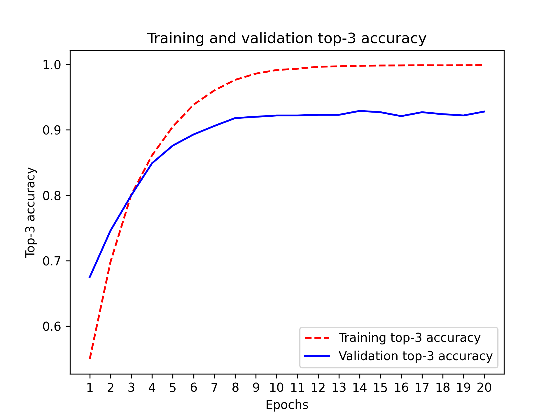
Like last time, we'll also monitor accuracy. However, accuracy is a bit of a crude metric in this case: if the model has the correct class as its second choice for a given sample, with an incorrect first choice, the model will still have an accuracy of zero on that sample — even though such a model would be much better than a random guess. A more nuanced metric in this case is top-k accuracy, such as top-3 or top-5 accuracy. It measures whether the correct class was among the top-k predictions of the model. Let's add top-3 accuracy to our model.

top_3_accuracy = keras.metrics.TopKCategoricalAccuracy(
    k=3, name="top_3_accuracy"
)
model.compile(
    optimizer="adam",
    loss="categorical_crossentropy",
    metrics=["accuracy", top_3_accuracy],
)

Validating your approach

Let's set apart 1,000 samples in the training data to use as a validation set.

x_val = x_train[:1000]
partial_x_train = x_train[1000:]
y_val = y_train[:1000]
partial_y_train = y_train[1000:]

Now, let's train the model for 20 epochs.

history = model.fit(
    partial_x_train,
    partial_y_train,
    epochs=20,
    batch_size=512,
    validation_data=(x_val, y_val),
)

And finally, let's display its loss and accuracy curves (see figures 4.6 and 4.7).

loss = history.history["loss"]
val_loss = history.history["val_loss"]
epochs = range(1, len(loss) + 1)
plt.plot(epochs, loss, "r--", label="Training loss")
plt.plot(epochs, val_loss, "b", label="Validation loss")
plt.title("Training and validation loss")
plt.xlabel("Epochs")
plt.xticks(epochs)
plt.ylabel("Loss")
plt.legend()
plt.show()

plt.clf()
acc = history.history["accuracy"]
val_acc = history.history["val_accuracy"]
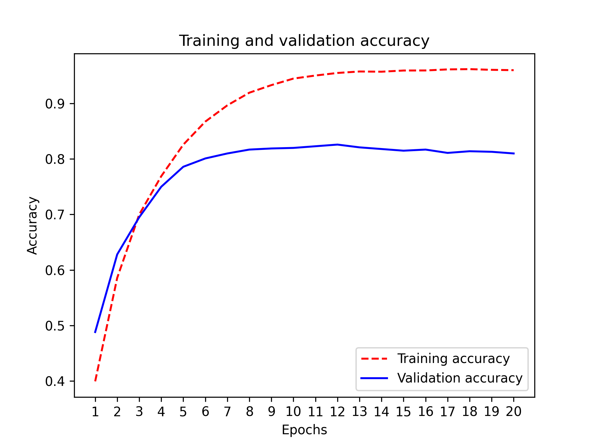
plt.plot(epochs, acc, "r--", label="Training accuracy")
plt.plot(epochs, val_acc, "b", label="Validation accuracy")
plt.title("Training and validation accuracy")
plt.xlabel("Epochs")
plt.xticks(epochs)
plt.ylabel("Accuracy")
plt.legend()
plt.show()

plt.clf()
acc = history.history["top_3_accuracy"]
val_acc = history.history["val_top_3_accuracy"]
plt.plot(epochs, acc, "r--", label="Training top-3 accuracy")
plt.plot(epochs, val_acc, "b", label="Validation top-3 accuracy")
plt.title("Training and validation top-3 accuracy")
plt.xlabel("Epochs")
plt.xticks(epochs)
plt.ylabel("Top-3 accuracy")
plt.legend()
plt.show()

The model begins to overfit after nine epochs. Let's train a new model from scratch for nine epochs and then evaluate it on the test set.

model = keras.Sequential(
    [
        layers.Dense(64, activation="relu"),
        layers.Dense(64, activation="relu"),
        layers.Dense(46, activation="softmax"),
    ]
)
model.compile(
    optimizer="adam",
    loss="categorical_crossentropy",
    metrics=["accuracy"],
)
model.fit(
    x_train,
    y_train,
    epochs=9,
    batch_size=512,
)
results = model.evaluate(x_test, y_test)

Here are the final results:

>>> results
[0.9565213431445807, 0.79697239536954589]

This approach reaches an accuracy of approximately 80%. With a balanced binary classification problem, the accuracy reached by a purely random classifier would be 50%. But in this case, we have 46 classes, and they may not be equally represented. What would be the accuracy of a random baseline? We could try quickly implementing one to check this empirically:

>>> import copy
>>> test_labels_copy = copy.copy(test_labels)
>>> np.random.shuffle(test_labels_copy)
>>> hits_array = np.array(test_labels == test_labels_copy)
>>> hits_array.mean()
0.18655387355298308

As you can see, a random classifier would score around 19% classification accuracy, so the results of our model seem pretty good in that light.

Generating predictions on new data

Calling the model's predict method on new samples returns a class probability distribution over all 46 topics for each sample. Let's generate topic predictions for all of the test data:

predictions = model.predict(x_test)

Each entry in "predictions" is a vector of length 46:

>>> predictions[0].shape
(46,)

The coefficients in this vector sum to 1, as they form a probability distribution:

>>> np.sum(predictions[0])
1.0

The largest entry is the predicted class — the class with the highest probability:

>>> np.argmax(predictions[0])
4

A different way to handle the labels and the loss

We mentioned earlier that another way to encode the labels would be to leave them untouched as integer tensors, like this:

y_train = train_labels
y_test = test_labels

The only thing this approach would change is the choice of the loss function. The loss function used in listing 4.22, categorical_crossentropy, expects the labels to follow a categorical encoding. With integer labels, you should use sparse_categorical_crossentropy:

model.compile(
    optimizer="adam",
    loss="sparse_categorical_crossentropy",
    metrics=["accuracy"],
)

This new loss function is still mathematically the same as categorical_crossentropy; it just has a different interface.

The importance of having sufficiently large intermediate layers

We mentioned earlier that because the final outputs are 46-dimensional, you should avoid intermediate layers with much fewer than 46 units. Now let's see what happens when you introduce an information bottleneck by having intermediate layers that are significantly less than 46-dimensional: for example, 4-dimensional.

model = keras.Sequential(
    [
        layers.Dense(64, activation="relu"),
        layers.Dense(4, activation="relu"),
        layers.Dense(46, activation="softmax"),
    ]
)
model.compile(
    optimizer="adam",
    loss="categorical_crossentropy",
    metrics=["accuracy"],
)
model.fit(
    partial_x_train,
    partial_y_train,
    epochs=20,
    batch_size=128,
    validation_data=(x_val, y_val),
)

The model now peaks at approximately 71% validation accuracy, an 8% absolute drop. This drop is mostly due to the fact that you're trying to compress a lot of information (enough information to recover the separation hyperplanes of 46 classes) into an intermediate space that is too low-dimensional. The model is able to cram most of the necessary information into these four-dimensional representations, but not all of it.

Further experiments

Like in the previous example, we encourage you to try out the following experiments to train your intuition about the kind of configuration decisions you have to make with such models:

• Try using larger or smaller layers: 32 units, 128 units, and so on.
• You used two intermediate layers before the final softmax classification layer. Now try using a single intermediate layer, or three intermediate layers.

Wrapping up

Here's what you should take away from this example:

• If you're trying to classify data points among N classes, your model should end with a Dense layer of size N.

• In a single-label, multiclass classification problem, your model should end with a softmax activation so that it will output a probability distribution over the N output classes.

• Categorical crossentropy is almost always the loss function you should use for such problems. It minimizes the distance between the probability distributions output by the model and the true distribution of the targets.

• There are two ways to handle labels in multiclass classification:
  • Encoding the labels via categorical encoding (also known as one-hot encoding) and using categorical_crossentropy as a loss function
  • Encoding the labels as integers and using the sparse_categorical_crossentropy loss function

• If you need to classify data into a large number of categories, you should avoid creating information bottlenecks in your model due to intermediate layers that are too small.

Predicting house prices: a regression example

The two previous examples were considered classification problems, where the goal was to predict a single discrete label of an input data point. Another common type of machine learning problem is regression, which consists of predicting a continuous value instead of a discrete label: for instance, predicting the temperature tomorrow given meteorological data, or predicting the time that a software project will take to complete given its specifications.

The California Housing Price dataset

You'll attempt to predict the median price of homes in different areas of California, based on data from the 1990 census.

Each data point in the dataset represents information about a "block group," a group of homes located in the same area. You can think of it as a district. This dataset has two versions, the "small" version with just 600 districts, and the "large" version with 20,640 districts. Let's use the small version, because real-world datasets can often be tiny, and you need to know how to handle such cases.

For each district, we know

• The longitude and latitude of the approximate geographic center of the area.
• The median age of houses in the district.
• The population of the district. The districts are pretty small: the average population is 1,425.5.
• The total number of households.
• The median income of those households.
• The total number of rooms in the district, across all homes located there. This is typically in the low thousands.
• The total number of bedrooms in the district.

That's eight variables in total (longitude and latitude counts as two variables). The goal is to use these variables to predict the median value of the houses in the district. Let's get started by loading the data.

from keras.datasets import california_housing

# Make sure to pass version="small" to get the right dataset.
(train_data, train_targets), (test_data, test_targets) = (
    california_housing.load_data(version="small")
)

Let's look at the data:

>>> train_data.shape
(480, 8)
>>> test_data.shape
(120, 8)

As you can see, we have 480 training samples and 120 test samples, each with 8 numerical features. The targets are the median values of homes in the district considered, in dollars:

>>> train_targets
array([252300., 146900., 290900., ..., 140500., 217100.],
      dtype=float32)

The prices are between $60,000 and $500,000. If that sounds cheap, remember that this was in 1990, and these prices aren't adjusted for inflation.

Preparing the data

It would be problematic to feed into a neural network values that all take wildly different ranges. The model might be able to automatically adapt to such heterogeneous data, but it would definitely make learning more difficult. A widespread best practice to deal with such data is to do feature-wise normalization: for each feature in the input data (a column in the input data matrix), you subtract the mean of the feature and divide by the standard deviation, so that the feature is centered around 0 and has a unit standard deviation. This is easily done in NumPy.

mean = train_data.mean(axis=0)
std = train_data.std(axis=0)
x_train = (train_data - mean) / std
x_test = (test_data - mean) / std

Note that the quantities used for normalizing the test data are computed using the training data. You should never use in your workflow any quantity computed on the test data, even for something as simple as data normalization.

In addition, we should also scale the targets. Our normalized inputs have their value in a small range close to 0, and our model's weights are initialized with small random values. This means that our model's prediction will also be small values when we start training. If the targets are in the range 60,000-500,000, the model is going to need very large weight values to output those. With a small learning rate, it would take a very long time to get there. The simplest fix is to divide all target values by 100,000, so that the smallest target becomes 0.6, and the largest becomes 5. We can then convert the model's predictions back to dollar values by multiplying them by 100,000 accordingly.

y_train = train_targets / 100000
y_test = test_targets / 100000

Building your model

Because so few samples are available, you'll use a very small model with two intermediate layers, each with 64 units. In general, the less training data you have, the worse overfitting will be, and using a small model is one way to mitigate overfitting.

def get_model():
    # Because you'll need to instantiate the same model multiple times,
    # you use a function to construct it.
    model = keras.Sequential(
        [
            layers.Dense(64, activation="relu"),
            layers.Dense(64, activation="relu"),
            layers.Dense(1),
        ]
    )
    model.compile(
        optimizer="adam",
        loss="mean_squared_error",
        metrics=["mean_absolute_error"],
    )
    return model

The model ends with a single unit and no activation: it will be a linear layer. This is a typical setup for scalar regression — a regression where you're trying to predict a single continuous value. Applying an activation function would constrain the range the output can take; for instance, if you applied a sigmoid activation function to the last layer, the model could only learn to predict values between 0 and 1. Here, because the last layer is purely linear, the model is free to learn to predict values in any range.

Note that you compile the model with the mean_squared_error loss function — mean squared error, the square of the difference between the predictions and the targets. This is a widely used loss function for regression problems.

You're also monitoring a new metric during training: mean absolute error (MAE). It's the absolute value of the difference between the predictions and the targets. For instance, an MAE of 0.5 on this problem would mean your predictions are off by $50,000 on average (remember the target scaling of factor 100,000).

Validating your approach using K-fold validation

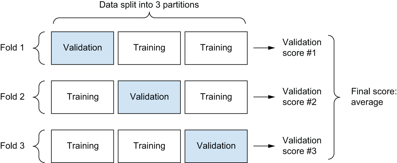
To evaluate your model while you keep adjusting its parameters (such as the number of epochs used for training), you could split the data into a training set and a validation set, as you did in the previous examples. But because you have so few data points, the validation set would end up being very small (for instance, about 100 examples). As a consequence, the validation scores might change a lot depending on which data points you chose to use for validation and which you chose for training: the validation scores might have a high variance with regard to the validation split. This would prevent you from reliably evaluating your model.

The best practice in such situations is to use K-fold cross-validation (see figure 4.9). It consists of splitting the available data into K partitions (typically K = 4 or 5), instantiating K identical models, and training each one on K – 1 partitions while evaluating on the remaining partition. The validation score for the model used is then the average of the K validation scores obtained. In terms of code, this is straightforward.

k = 4
num_val_samples = len(x_train) // k
num_epochs = 50
all_scores = []
for i in range(k):
    print(f"Processing fold #{i + 1}")
    # Prepares the validation data: data from partition #k
    fold_x_val = x_train[i * num_val_samples : (i + 1) * num_val_samples]
    fold_y_val = y_train[i * num_val_samples : (i + 1) * num_val_samples]
    # Prepares the training data: data from all other partitions
    fold_x_train = np.concatenate(
        [x_train[: i * num_val_samples], x_train[(i + 1) * num_val_samples :]],
        axis=0,
    )
    fold_y_train = np.concatenate(
        [y_train[: i * num_val_samples], y_train[(i + 1) * num_val_samples :]],
        axis=0,
    )
    # Builds the Keras model (already compiled)
    model = get_model()
    # Trains the model
    model.fit(
        fold_x_train,
        fold_y_train,
        epochs=num_epochs,
        batch_size=16,
        verbose=0,
    )
    # Evaluates the model on the validation data
    scores = model.evaluate(fold_x_val, fold_y_val, verbose=0)
    val_loss, val_mae = scores
    all_scores.append(val_mae)

Running this with num_epochs = 50 yields the following results:

>>> [round(value, 3) for value in all_scores]
[0.298, 0.349, 0.232, 0.305]
>>> round(np.mean(all_scores), 3)
0.296

The different runs do indeed show meaningfully different validation scores, from 0.232 to 0.349. The average (0.296) is a much more reliable metric than any single score — that's the entire point of K-fold cross-validation. In this case, you're off by $29,600 on average, which is significant considering that the prices range from $60,000 to $500,000.

Let's try training the model a bit longer: 200 epochs. To keep a record of how well the model does at each epoch, you'll modify the training loop to save the per-epoch validation score log.

k = 4
num_val_samples = len(x_train) // k
num_epochs = 200
all_mae_histories = []
for i in range(k):
    print(f"Processing fold #{i + 1}")
    # Prepares the validation data: data from partition #k
    fold_x_val = x_train[i * num_val_samples : (i + 1) * num_val_samples]
    fold_y_val = y_train[i * num_val_samples : (i + 1) * num_val_samples]
    # Prepares the training data: data from all other partitions
    fold_x_train = np.concatenate(
        [x_train[: i * num_val_samples], x_train[(i + 1) * num_val_samples :]],
        axis=0,
    )
    fold_y_train = np.concatenate(
        [y_train[: i * num_val_samples], y_train[(i + 1) * num_val_samples :]],
        axis=0,
    )
    # Builds the Keras model (already compiled)
    model = get_model()
    # Trains the model
    history = model.fit(
        fold_x_train,
        fold_y_train,
        validation_data=(fold_x_val, fold_y_val),
        epochs=num_epochs,
        batch_size=16,
        verbose=0,
    )
    mae_history = history.history["val_mean_absolute_error"]
    all_mae_histories.append(mae_history)

You can then compute the average of the per-epoch mean absolute error (MAE) scores for all folds.

average_mae_history = [
    np.mean([x[i] for x in all_mae_histories]) for i in range(num_epochs)
]

Let's plot this; see figure 4.10.

epochs = range(1, len(average_mae_history) + 1)
plt.plot(epochs, average_mae_history)
plt.xlabel("Epochs")
plt.ylabel("Validation MAE")
plt.show()

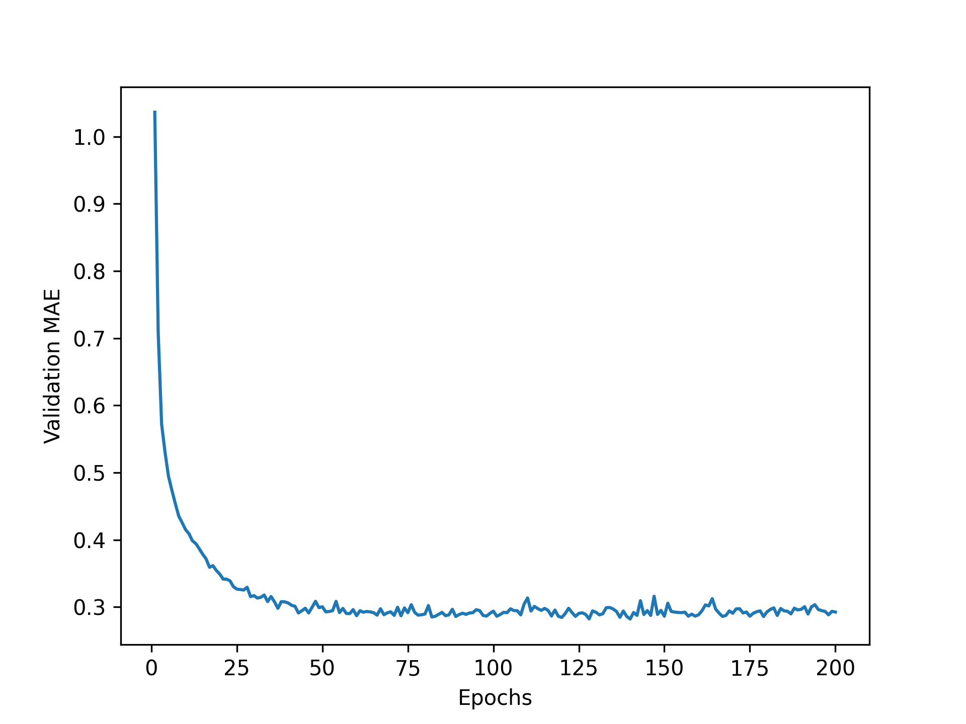
It may be a little difficult to read the plot due to a scaling issue: the validation MAE for the first few epochs is dramatically higher than the values that follow. Let's omit the first 10 data points, which are on a different scale than the rest of the curve:

truncated_mae_history = average_mae_history[10:]
epochs = range(10, len(truncated_mae_history) + 10)
plt.plot(epochs, truncated_mae_history)
plt.xlabel("Epochs")
plt.ylabel("Validation MAE")
plt.show()

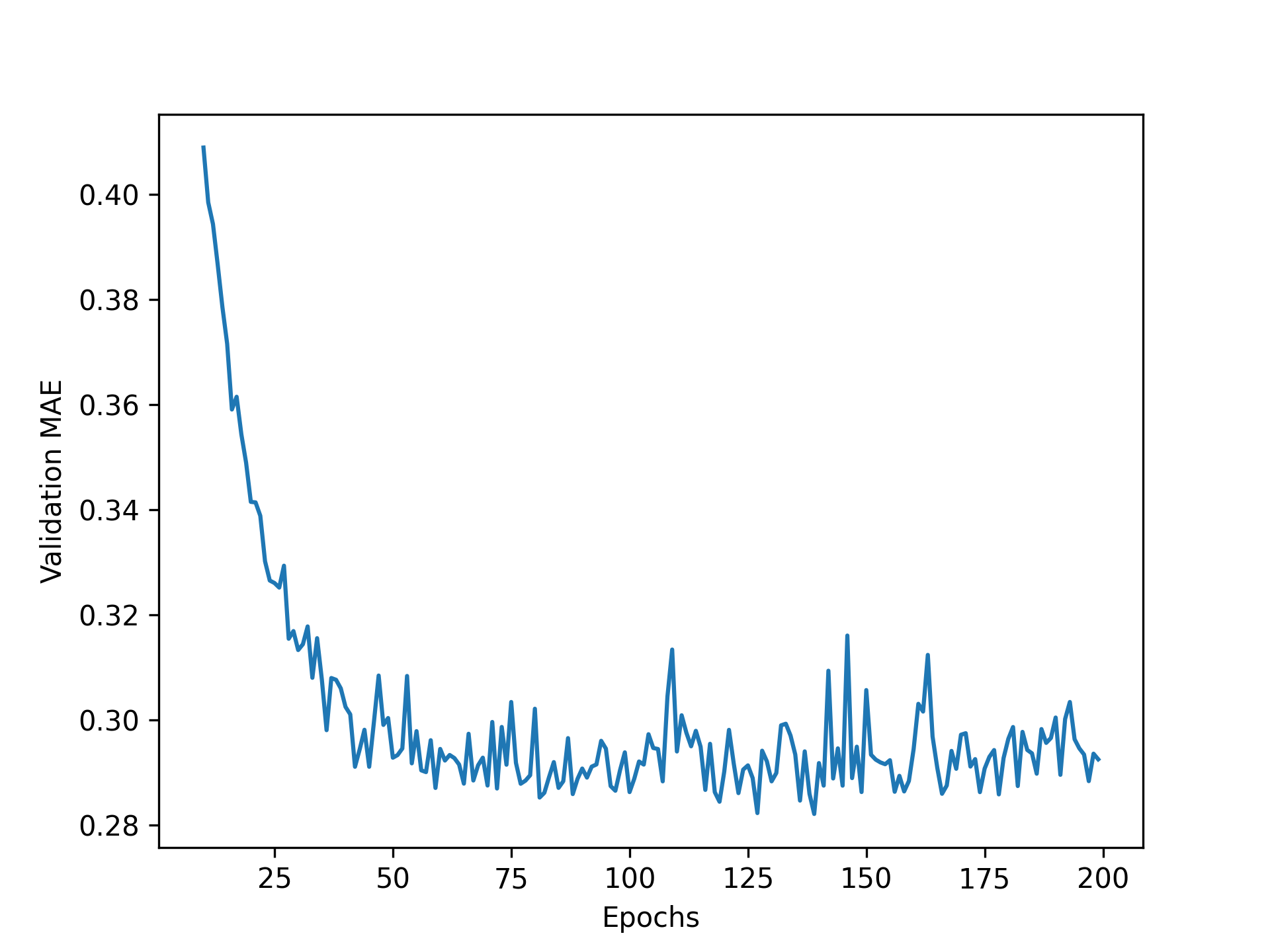
According to this plot, validation MAE stops improving significantly after 120-140 epochs (this number includes the 10 epochs we omitted). Past that point, you start overfitting.

Once you're finished tuning other parameters of the model (in addition to the number of epochs, you could also adjust the size of the intermediate layers), you can train a final production model on all of the training data, with the best parameters, and then look at its performance on the test data.

# Gets a fresh, compiled model
model = get_model()
# Trains it on the entirety of the data
model.fit(x_train, y_train, epochs=130, batch_size=16, verbose=0)
test_mean_squared_error, test_mean_absolute_error = model.evaluate(
    x_test, y_test
)

Here's the final result:

>>> round(test_mean_absolute_error, 3)
0.31

We're still off by about $31,000 on average.

Generating predictions on new data

When calling predict() on our binary classification model, we retrieved a scalar score between 0 and 1 for each input sample. With our multi-class classification model, we retrieved a probability distribution over all classes for each sample. Now, with this scalar regression model, predict() returns the model's guess for the sample's price in hundreds of thousands of dollars:

>>> predictions = model.predict(x_test)
>>> predictions[0]
array([2.834494], dtype=float32)

The first district in the test set is predicted to have an average home price of about $283,000.

Wrapping up

Here's what you should take away from this scalar regression example:

• Regression is done using a different loss function than what we used for classification. Mean squared error (MSE) is a loss function commonly used for regression.

• Similarly, evaluation metrics to be used for regression differ from those used for classification; naturally, the concept of accuracy doesn't apply for regression. A common regression metric is MAE.

• When features in the input data have values in different ranges, each feature should be scaled independently as a preprocessing step.

• When there is little data available, using K-fold validation is a great way to reliably evaluate a model.

• When little training data is available, it's preferable to use a small model with few intermediate layers (typically only one or two), in order to avoid severe overfitting.

Summary

• The three most common kinds of machine learning tasks on vector data are binary classification, multiclass classification, and scalar regression. Each task uses different loss functions:
  • binary_crossentropy for binary classification.
  • categorical_crossentropy for multiclass classification.
  • mean_squared_error for scalar regression.

• You'll usually need to preprocess raw data before feeding it into a neural network.

• When your data has features with different ranges, scale each feature independently as part of preprocessing.

• As training progresses, neural networks eventually begin to overfit and obtain worse results on never-before-seen data.

• If you don't have much training data, use a small model with only one or two intermediate layers, to avoid severe overfitting.

• If your data is divided into many categories, you may cause information bottlenecks if you make the intermediate layers too small.

• When you're working with little data, K-fold validation can help reliably evaluate your model.