Image classification

Computer vision was the first big success story of deep learning. It led to the initial rise of deep learning between 2011 and 2015. A type of deep learning called convolutional neural networks started getting remarkably good results on image classification competitions around that time, first with Dan Ciresan winning two niche competitions (the ICDAR 2011 Chinese character recognition competition and the IJCNN 2011 German traffic signs recognition competition) and then, more notably, in fall 2012, with Hinton's group winning the high-profile ImageNet large-scale visual recognition challenge. Many more promising results quickly started bubbling up in other computer vision tasks.

Interestingly, these early successes weren't quite enough to make deep learning mainstream at the time — it took a few years. The computer vision research community had spent many years investing in methods other than neural networks, and it wasn't quite ready to give up on them just because there was a new kid on the block. In 2013 and 2014, deep learning still faced intense skepticism from many senior computer vision researchers. It's only in 2016 that it finally became dominant. One author remembers exhorting an ex-professor, in February 2014, to pivot to deep learning. "It's the next big thing!" he would say. "Well, maybe it's just a fad," the professor would reply. By 2016, his entire lab was doing deep learning. There's no stopping an idea whose time has come.

Today, you're constantly interacting with deep learning-based vision models — via Google Photos, Google image search, the camera on your phone, YouTube, OCR software, and many more. These models are also at the heart of cutting-edge research in autonomous driving, robotics, AI-assisted medical diagnosis, autonomous retail checkout systems, and even autonomous farming.

This chapter introduces convolutional neural networks, also known as convnets or CNNs, the type of deep-learning model that is used by most computer vision applications. You'll learn to apply convnets to image classification problems — in particular, those involving small training datasets, which are the most common use case if you aren't a large tech company.

Introduction to convnets

We're about to dive into the theory of what convnets are and why they have been so successful at computer vision tasks. But first, let's take a practical look at a simple convnet example. It uses a convnet to classify MNIST digits, a task we performed in chapter 2 using a densely connected network (our test accuracy then was 97.8%). Even though the convnet will be basic, its accuracy will blow out of the water that of the densely connected model from chapter 2.

The following lines of code show you what a basic convnet looks like. It's a stack of Conv2D and MaxPooling2D layers. You'll see in a minute exactly what they do. We'll build the model using the Functional API, which we introduced in the previous chapter.

import keras
from keras import layers

inputs = keras.Input(shape=(28, 28, 1))
x = layers.Conv2D(filters=64, kernel_size=3, activation="relu")(inputs)
x = layers.MaxPooling2D(pool_size=2)(x)
x = layers.Conv2D(filters=128, kernel_size=3, activation="relu")(x)
x = layers.MaxPooling2D(pool_size=2)(x)
x = layers.Conv2D(filters=256, kernel_size=3, activation="relu")(x)
x = layers.GlobalAveragePooling2D()(x)
outputs = layers.Dense(10, activation="softmax")(x)
model = keras.Model(inputs=inputs, outputs=outputs)

Importantly, a convnet takes as input tensors of shape (image_height, image_width, image_channels) (not including the batch dimension). In this case, we'll configure the convnet to process inputs of size (28, 28, 1), which is the format of MNIST images.

Let's display the architecture of our convnet.

>>> model.summary()
Model: "functional"
┏━━━━━━━━━━━━━━━━━━━━━━━━━━━━━━━━━━━┳━━━━━━━━━━━━━━━━━━━━━━━━━━┳━━━━━━━━━━━━━━━┓
┃ Layer (type)                      ┃ Output Shape             ┃       Param # ┃
┡━━━━━━━━━━━━━━━━━━━━━━━━━━━━━━━━━━━╇━━━━━━━━━━━━━━━━━━━━━━━━━━╇━━━━━━━━━━━━━━━┩
│ input_layer (InputLayer)          │ (None, 28, 28, 1)        │             0 │
├───────────────────────────────────┼──────────────────────────┼───────────────┤
│ conv2d (Conv2D)                   │ (None, 26, 26, 64)       │           640 │
├───────────────────────────────────┼──────────────────────────┼───────────────┤
│ max_pooling2d (MaxPooling2D)      │ (None, 13, 13, 64)       │             0 │
├───────────────────────────────────┼──────────────────────────┼───────────────┤
│ conv2d_1 (Conv2D)                 │ (None, 11, 11, 128)      │        73,856 │
├───────────────────────────────────┼──────────────────────────┼───────────────┤
│ max_pooling2d_1 (MaxPooling2D)    │ (None, 5, 5, 128)        │             0 │
├───────────────────────────────────┼──────────────────────────┼───────────────┤
│ conv2d_2 (Conv2D)                 │ (None, 3, 3, 256)        │       295,168 │
├───────────────────────────────────┼──────────────────────────┼───────────────┤
│ global_average_pooling2d          │ (None, 256)              │             0 │
│ (GlobalAveragePooling2D)          │                          │               │
├───────────────────────────────────┼──────────────────────────┼───────────────┤
│ dense (Dense)                     │ (None, 10)               │         2,570 │
└───────────────────────────────────┴──────────────────────────┴───────────────┘
 Total params: 372,234 (1.42 MB)
 Trainable params: 372,234 (1.42 MB)
 Non-trainable params: 0 (0.00 B)

You can see that the output of every Conv2D and MaxPooling2D layer is a 3D tensor of shape (height, width, channels). The width and height dimensions tend to shrink as you go deeper in the model. The number of channels is controlled by the first argument passed to the Conv2D layers (64, 128, or 256).

After the last Conv2D layer, we end up with an output of shape (3, 3, 256) — a 3 x 3 feature map of 256 channels. The next step is to feed this output into a densely connected classifier like those you're already familiar with: a stack of Dense layers. These classifiers process vectors, which are 1D, whereas the current output is a rank-3 tensor. To bridge the gap, we flatten the 3D outputs to 1D with a GlobalAveragePooling2D layer before adding the Dense layers. This layer will take the average of each 3 x 3 feature map in the tensor of shape (3, 3, 256), resulting in an output vector of shape (256,).

Finally, we'll do 10-way classification, so our last layer has 10 outputs and a softmax activation.

Now, let's train the convnet on the MNIST digits. We'll reuse a lot of the code from the MNIST example in chapter 2. Because we're doing 10-way classification with a softmax output, we'll use the categorical crossentropy loss, and because our labels are integers, we'll use the sparse version, sparse_categorical_crossentropy.

from keras.datasets import mnist

(train_images, train_labels), (test_images, test_labels) = mnist.load_data()
train_images = train_images.reshape((60000, 28, 28, 1))
train_images = train_images.astype("float32") / 255
test_images = test_images.reshape((10000, 28, 28, 1))
test_images = test_images.astype("float32") / 255
model.compile(
    optimizer="adam",
    loss="sparse_categorical_crossentropy",
    metrics=["accuracy"],
)
model.fit(train_images, train_labels, epochs=5, batch_size=64)

Let's evaluate the model on the test data.

>>> test_loss, test_acc = model.evaluate(test_images, test_labels)
>>> print(f"Test accuracy: {test_acc:.3f}")
Test accuracy: 0.991

Whereas the densely connected model from chapter 2 had a test accuracy of 97.8%, the basic convnet has a test accuracy of 99.1%: we decreased the error rate by about 60% (relative). Not bad!

But why does this simple convnet work so well, compared to a densely connected model? To answer this, let's dive into what the Conv2D and MaxPooling2D layers do.

The convolution operation

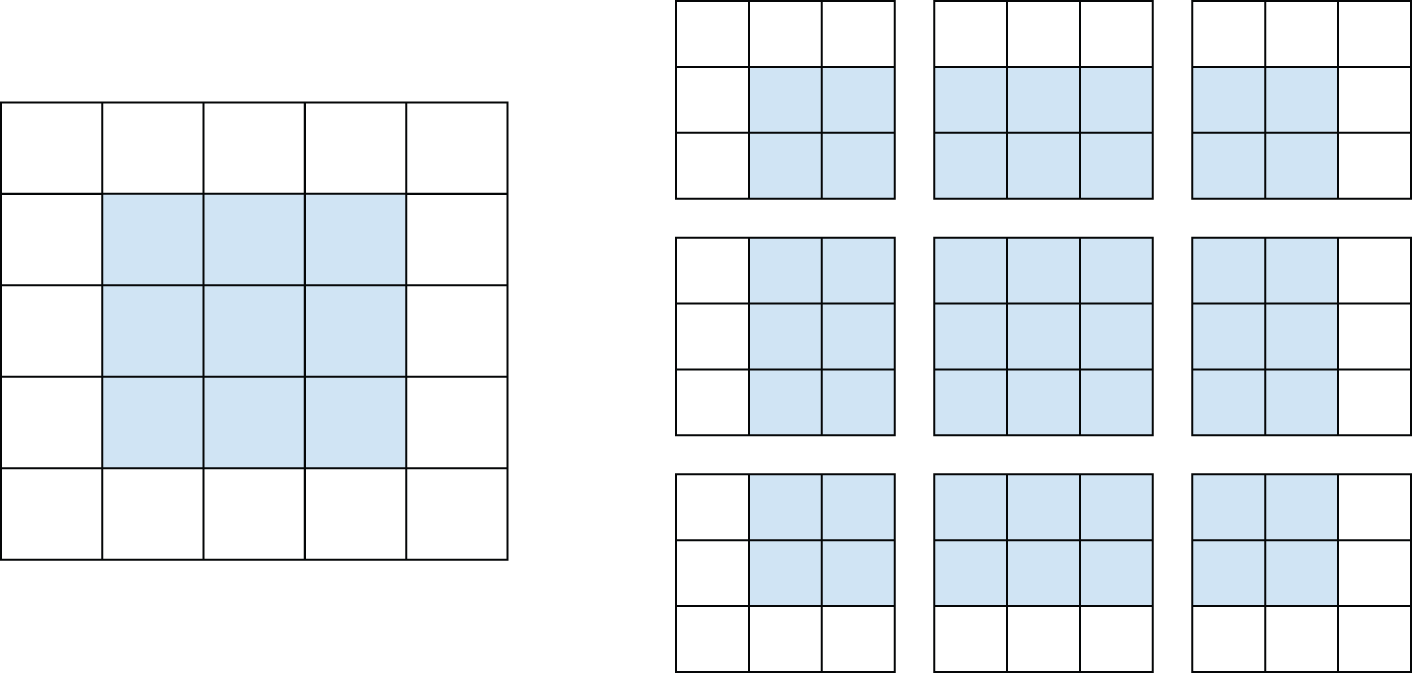
The fundamental difference between a densely connected layer and a convolution layer is this: Dense layers learn global patterns in their input feature space (for example, for a MNIST digit, patterns involving all pixels), whereas convolution layers learn local patterns (see figure 8.1): in the case of images, patterns found in small 2D windows of the inputs. In the previous example, these windows were all 3 × 3.

This key characteristic gives convnets two interesting properties:

• The patterns they learn are translation invariant. After learning a certain pattern in the lower-right corner of a picture, a convnet can recognize it anywhere: for example, in the upper-left corner. A densely connected model would have to learn the pattern anew if it appeared at a new location. This makes convnets data efficient when processing images — because the visual world is fundamentally translation invariant. They need fewer training samples to learn representations that have generalization power.

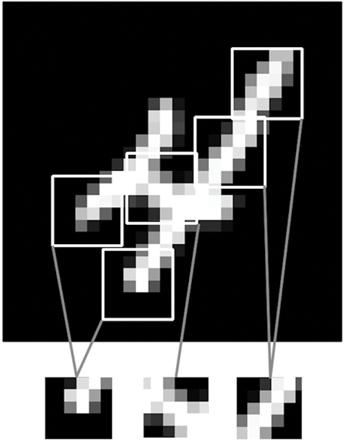
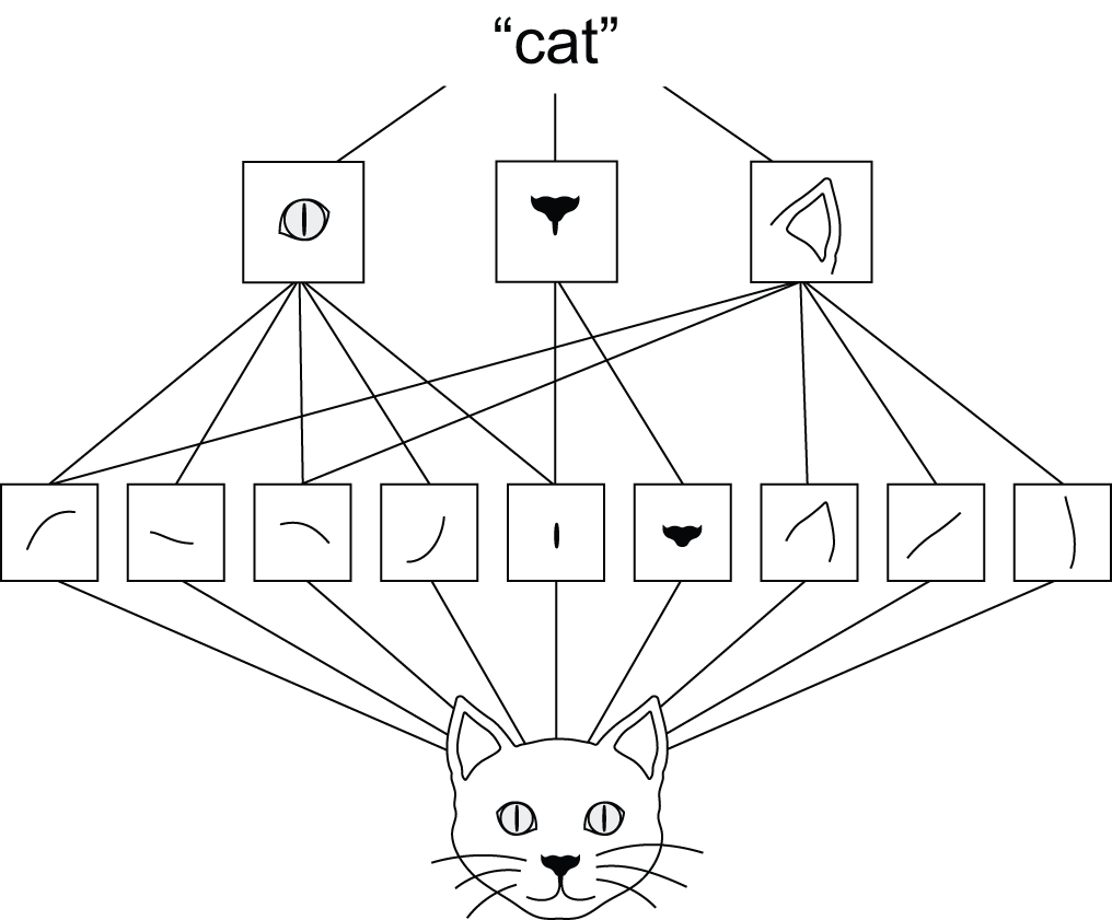
• They can learn spatial hierarchies of patterns (see figure 8.2). A first convolution layer will learn small local patterns such as edges, a second convolution layer will learn larger patterns made of the features of the first layers, and so on. This allows convnets to efficiently learn increasingly complex and abstract visual concepts — because the visual world is fundamentally spatially hierarchical.

Convolutions operate over rank-3 tensors, called feature maps, with two spatial axes (height and width) as well as a depth axis (also called the channels axis). For an RGB image, the dimension of the depth axis is 3, because the image has three color channels: red, green, and blue. For a black-and-white picture, like the MNIST digits, the depth is 1 (levels of gray). The convolution operation extracts patches from its input feature map and applies the same transformation to all of these patches, producing an output feature map. This output feature map is still a rank-3 tensor: it has a width and a height. Its depth can be arbitrary because the output depth is a parameter of the layer, and the different channels in that depth axis no longer stand for specific colors as in RGB input; rather, they stand for filters. Filters encode specific aspects of the input data: at a high level, a single filter could encode the concept "presence of a face in the input," for instance.

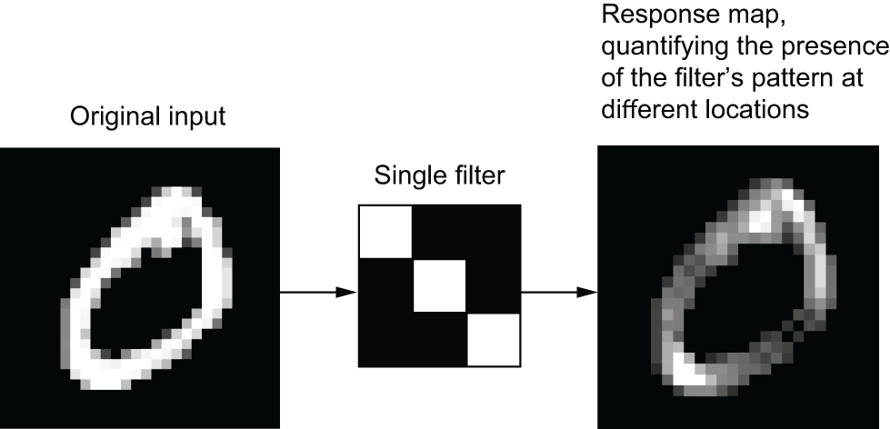
In the MNIST example, the first convolution layer takes a feature map of size (28, 28, 1) and outputs a feature map of size (26, 26, 64): it computes 64 filters over its input. Each of these 64 output channels contains a 26 × 26 grid of values, which is a response map of the filter over the input, indicating the response of that filter pattern at different locations in the input (see figure 8.3). That is what the term feature map means: every dimension in the depth axis is a feature (or filter), and the rank-2 tensor output[:, :, n] is the 2D spatial map of the response of this filter over the input.

Convolutions are defined by two key parameters:

• Size of the patches extracted from the inputs  — These are typically 3 × 3 or 5 × 5. In the example, they were 3 × 3, which is a common choice.

• Depth of the output feature map  — The number of filters computed by the convolution. The example started with a depth of 32 and ended with a depth of 64.

In Keras Conv2D layers, these parameters are the first arguments passed to the layer: Conv2D(output_depth, (window_height, window_width)).

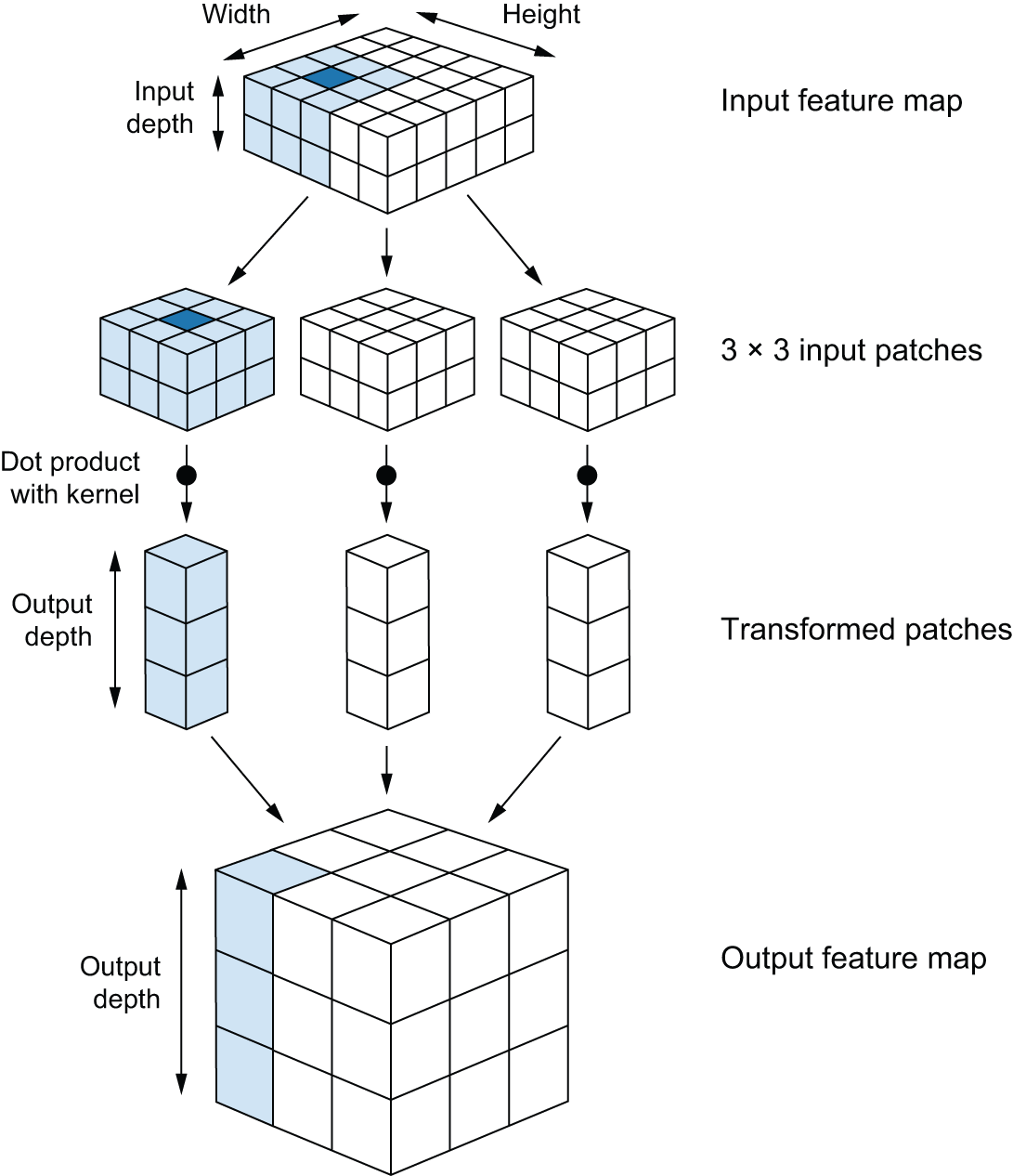
A convolution works by sliding these windows of size 3 × 3 or 5 × 5 over the 3D input feature map, stopping at every possible location, and extracting the 3D patch of surrounding features (shape (window_height, window_width, input_depth)). Each such 3D patch is then transformed into a 1D vector of shape (output_depth,), which is done via a tensor product with a learned weight matrix, called the convolution kernel — the same kernel is reused across every patch. All of these vectors (one per patch) are then spatially reassembled into a 3D output map of shape (height, width, output_depth). Every spatial location in the output feature map corresponds to the same location in the input feature map (for example, the lower-right corner of the output contains information about the lower-right corner of the input). For instance, with 3 × 3 windows, the vector output[i, j, :] comes from the 3D patch input[i-1:i+1, j-1:j+1, :]. The full process is detailed in figure 8.4.

Note that the output width and height may differ from the input width and height. They may differ for two reasons:

• Border effects, which can be countered by padding the input feature map
• The use of strides, which we'll define in a second

Let's take a deeper look at these notions.

Understanding border effects and padding

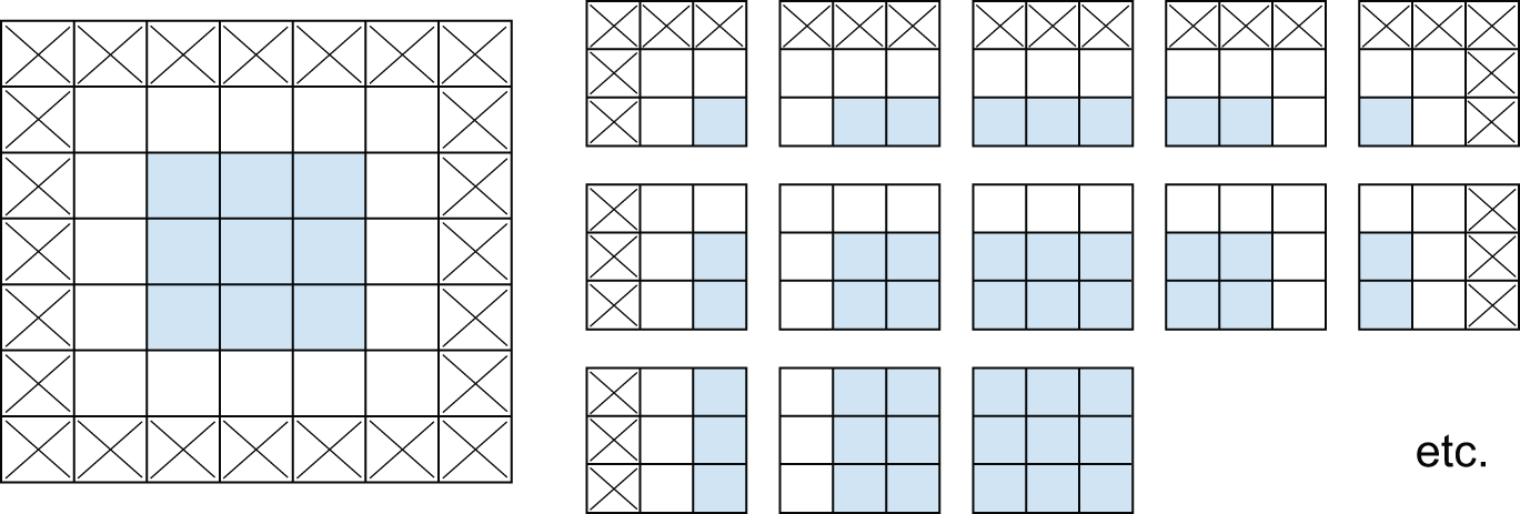
Consider a 5 × 5 feature map (25 tiles total). There are only 9 tiles around which you can center a 3 × 3 window, forming a 3 × 3 grid (see figure 8.5). Hence, the output feature map will be 3 × 3. It shrinks a little: by exactly two tiles alongside each dimension, in this case. You can see this border effect in action in the earlier example: you start with 28 × 28 inputs, which become 26 × 26 after the first convolution layer.

If you want to get an output feature map with the same spatial dimensions as the input, you can use padding. Padding consists of adding an appropriate number of rows and columns on each side of the input feature map so as to make it possible to fit centered convolution windows around every input tile. For a 3 × 3 window, you add one column on the right, one column on the left, one row at the top, and one row at the bottom. For a 5 × 5 window, you add two rows (see figure 8.6).

In Conv2D layers, padding is configurable via the padding argument, which takes two values: "valid", which means no padding (only valid window locations will be used); and "same", which means "pad in such a way as to have an output with the same width and height as the input." The padding argument defaults to "valid".

Understanding convolution strides

The other factor that can influence output size is the notion of strides. The description of convolution so far has assumed that the center tiles of the convolution windows are all contiguous. But the distance between two successive windows is a parameter of the convolution, called its stride, which defaults to 1. It's possible to have strided convolutions: convolutions with a stride higher than 1. In figure 8.7, you can see the patches extracted by a 3 × 3 convolution with stride 2 over a 5 × 5 input (without padding)

Using stride 2 means the width and height of the feature map are downsampled by a factor of 2 (in addition to any changes induced by border effects). Strided convolutions are rarely used in classification models, but they come in handy for some types of models, as you will find out in the next chapter.

In classification models, instead of strides, we tend to use the max-pooling operation to downsample feature maps — which you saw in action in our first convnet example. Let's look at it in more depth.

The max-pooling operation

In the convnet example, you may have noticed that the size of the feature maps is halved after every MaxPooling2D layer. For instance, before the first MaxPooling2D layers, the feature map is 26 × 26, but the max-pooling operation halves it to 13 × 13. That's the role of max pooling: to aggressively downsample feature maps, much like strided convolutions.

Max pooling consists of extracting windows from the input feature maps and outputting the max value of each channel. It's conceptually similar to convolution, except that instead of transforming local patches via a learned linear transformation (the convolution kernel), they're transformed via a hardcoded max tensor operation. A big difference from convolution is that max pooling is usually done with 2 × 2 windows and stride 2 to downsample the feature maps by a factor of 2. On the other hand, convolution is typically done with 3 × 3 windows and no stride (stride 1).

Why downsample feature maps this way? Why not remove the max-pooling layers and keep fairly large feature maps all the way up? Let's look at this option. Our model would then look like this.

inputs = keras.Input(shape=(28, 28, 1))
x = layers.Conv2D(filters=64, kernel_size=3, activation="relu")(inputs)
x = layers.Conv2D(filters=128, kernel_size=3, activation="relu")(x)
x = layers.Conv2D(filters=256, kernel_size=3, activation="relu")(x)
x = layers.GlobalAveragePooling2D()(x)
outputs = layers.Dense(10, activation="softmax")(x)
model_no_max_pool = keras.Model(inputs=inputs, outputs=outputs)

Here's a summary of the model:

>>> model_no_max_pool.summary()
Model: "functional_1"
┏━━━━━━━━━━━━━━━━━━━━━━━━━━━━━━━━━━━┳━━━━━━━━━━━━━━━━━━━━━━━━━━┳━━━━━━━━━━━━━━━┓
┃ Layer (type)                      ┃ Output Shape             ┃       Param # ┃
┡━━━━━━━━━━━━━━━━━━━━━━━━━━━━━━━━━━━╇━━━━━━━━━━━━━━━━━━━━━━━━━━╇━━━━━━━━━━━━━━━┩
│ input_layer_1 (InputLayer)        │ (None, 28, 28, 1)        │             0 │
├───────────────────────────────────┼──────────────────────────┼───────────────┤
│ conv2d_3 (Conv2D)                 │ (None, 26, 26, 64)       │           640 │
├───────────────────────────────────┼──────────────────────────┼───────────────┤
│ conv2d_4 (Conv2D)                 │ (None, 24, 24, 128)      │        73,856 │
├───────────────────────────────────┼──────────────────────────┼───────────────┤
│ conv2d_5 (Conv2D)                 │ (None, 22, 22, 256)      │       295,168 │
├───────────────────────────────────┼──────────────────────────┼───────────────┤
│ global_average_pooling2d_1        │ (None, 256)              │             0 │
│ (GlobalAveragePooling2D)          │                          │               │
├───────────────────────────────────┼──────────────────────────┼───────────────┤
│ dense_1 (Dense)                   │ (None, 10)               │         2,570 │
└───────────────────────────────────┴──────────────────────────┴───────────────┘
 Total params: 372,234 (1.42 MB)
 Trainable params: 372,234 (1.42 MB)
 Non-trainable params: 0 (0.00 B)

What's wrong with this setup? Two things:

• It isn't conducive to learning a spatial hierarchy of features. The 3 × 3 windows in the third layer will only contain information coming from 7 × 7 windows in the initial input. The high-level patterns learned by the convnet will still be very small with regard to the initial input, which may not be enough to learn to classify digits (try recognizing a digit by only looking at it through windows that are 7 × 7 pixels!). We need the features from the last convolution layer to contain information about the totality of the input.

• The final feature map has dimensions 22 × 22. That's huge — when you take the average of each 22 x 22 feature map, you are going to be destroying a lot of information compared to when your feature maps were only 3 x 3.

In short, the reason to use downsampling is to reduce the size of the feature maps, making the information they contain increasingly less spatially distributed and increasingly contained in the channels, while also inducing spatial-filter hierarchies by making successive convolution layers "look" at increasingly large windows (in terms of the fraction of the original input image they cover).

Note that max pooling isn't the only way you can achieve such downsampling. As you already know, you can also use strides in the prior convolution layer. And you can use average pooling instead of max pooling, where each local input patch is transformed by taking the average value of each channel over the patch, rather than the max. But max pooling tends to work better than these alternative solutions. In a nutshell, the reason is that features tend to encode the spatial presence of some pattern or concept over the different tiles of the feature map (hence, the term feature map), and it's more informative to look at the maximal presence of different features than at their average presence. So the most reasonable subsampling strategy is to first produce dense maps of features (via unstrided convolutions) and then look at the maximal activation of the features over small patches, rather than looking at sparser windows of the inputs (via strided convolutions) or averaging input patches, which could cause you to miss or dilute feature-presence information.

At this point, you should understand the basics of convnets — feature maps, convolution, and max pooling — and you know how to build a small convnet to solve a toy problem such as MNIST digits classification. Now let's move on to more useful, practical applications.

Training a convnet from scratch on a small dataset

Having to train an image-classification model using very little data is a common situation, which you'll likely encounter in practice if you ever do computer vision in a professional context. A "few" samples can mean anywhere from a few hundred to a few tens of thousands of images. As a practical example, we'll focus on classifying images as dogs or cats. We'll work with a dataset containing 5,000 pictures of cats and dogs (2,500 cats, 2,500 dogs), taken from the original Kaggle dataset. We'll use 2,000 pictures for training, 1,000 for validation, and 2,000 for testing.

In this section, we'll review one basic strategy to tackle this problem: training a new model from scratch using what little data you have. We'll start by naively training a small convnet on the 2,000 training samples, without any regularization, to set a baseline for what can be achieved. This will get us to a classification accuracy of about 80%. At that point, the main issue will be overfitting. Then we'll introduce data augmentation, a powerful technique for mitigating overfitting in computer vision. By using data augmentation, we'll improve the model to reach a test accuracy of about 84%.

In the next section, we'll review two more essential techniques for applying deep learning to small datasets: feature extraction with a pretrained model and fine-tuning a pretrained model (which will get us to a final accuracy of 98.5%). Together, these three strategies — training a small model from scratch, doing feature extraction using a pretrained model, and fine-tuning a pretrained model — will constitute your future toolbox for tackling the problem of performing image classification with small datasets.

The relevance of deep learning for small-data problems

What qualifies as "enough samples" to train a model is relative — relative to the size and depth of the model you're trying to train, for starters. It isn't possible to train a convnet to solve a complex problem with just a few tens of samples, but a few hundred can potentially suffice if the model is small and well regularized and the task is simple. Because convnets learn local, translation-invariant features, they're highly data efficient on perceptual problems. Training a convnet from scratch on a very small image dataset will still yield reasonable results despite a relative lack of data, without the need for any custom feature engineering. You'll see this in action in this section.

What's more, deep-learning models are by nature highly repurposable: you can take, say, an image-classification or speech-to-text model trained on a large-scale dataset and reuse it on a significantly different problem with only minor changes. Specifically, in the case of computer vision, many pretrained classification models are publicly available for download and can be used to bootstrap powerful vision models out of very little data. This is one of the greatest strengths of deep learning: feature reuse. You'll explore this in the next section.

Let's start by getting our hands on the data.

Downloading the data

The Dogs vs. Cats dataset that we will use isn't packaged with Keras. It was made available by Kaggle as part of a computer-vision competition in late 2013, back when convnets weren't mainstream. You can download the original dataset from www.kaggle.com/c/dogs-vs-cats/data (you'll need to create a Kaggle account if you don't already have one — don't worry, the process is painless). You can also use the Kaggle API to download the dataset in Colab.

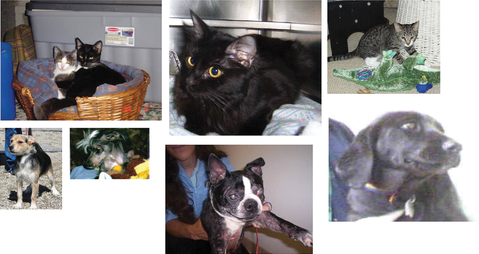
The pictures in our dataset are medium-resolution color JPEGs. Figure 8.8 shows some examples.

Unsurprisingly, the original dogs-versus-cats Kaggle competition, all the way back in 2013, was won by entrants who used convnets. The best entries achieved up to 95% accuracy. In this example, we will get fairly close to this accuracy (in the next section), even though we will train our models on less than 10% of the data that was available to the competitors.

This dataset contains 25,000 images of dogs and cats (12,500 from each class) and is 543 MB (compressed). After downloading and uncompressing the data, we'll create a new dataset containing three subsets: a training set with 1,000 samples of each class, a validation set with 500 samples of each class, and a test set with 1,000 samples of each class. Why do this? Because many of the image datasets you'll encounter in your career only contain a few thousand samples, not tens of thousands. Having more data available would make the problem easier — so it's good practice to learn with a small dataset.

The sub-sampled dataset we will work with will have the following directory structure:

dogs_vs_cats_small/
...train/
# Contains 1,000 cat images
......cat/
# Contains 1,000 dog images
......dog/
...validation/
# Contains 500 cat images
......cat/
# Contains 500 dog images
......dog/
...test/
# Contains 1,000 cat images
......cat/
# Contains 1,000 dog images
......dog/

Let's make it happen in a couple calls to shutil, a Python library for running shell-like commands.

import os, shutil, pathlib

# Path to the directory where the original dataset was uncompressed
original_dir = pathlib.Path("train")
# Directory where we will store our smaller dataset
new_base_dir = pathlib.Path("dogs_vs_cats_small")

# Utility function to copy cat (respectively, dog) images from index
# `start_index` to index `end_index` to the subdirectory
# `new_base_dir/{subset_name}/cat` (respectively, dog). "subset_name"
# will be either "train," "validation," or "test."
def make_subset(subset_name, start_index, end_index):
    for category in ("cat", "dog"):
        dir = new_base_dir / subset_name / category
        os.makedirs(dir)
        fnames = [f"{category}.{i}.jpg" for i in range(start_index, end_index)]
        for fname in fnames:
            shutil.copyfile(src=original_dir / fname, dst=dir / fname)

# Creates the training subset with the first 1,000 images of each
# category
make_subset("train", start_index=0, end_index=1000)
# Creates the validation subset with the next 500 images of each
# category
make_subset("validation", start_index=1000, end_index=1500)
# Creates the test subset with the next 1,000 images of each category
make_subset("test", start_index=1500, end_index=2500)

So we now have 2,000 training images, 1,000 validation images, and 2,000 test images. Each split contains the same number of samples from each class: this is a balanced binary-classification problem, which means classification accuracy will be an appropriate measure of success.

Building your model

We will reuse the same general model structure you saw in the first example: the convnet will be a stack of alternated Conv2D (with relu activation) and MaxPooling2D layers.

But because we're dealing with bigger images and a more complex problem, we'll make our model larger, accordingly: it will have two more Conv2D + MaxPooling2D stages. This serves both to augment the capacity of the model and to further reduce the size of the feature maps so they aren't overly large when we reach the pooling layer. Here, because we start from inputs of size 180 × 180 pixels (a somewhat arbitrary choice), we end up with feature maps of size 7 × 7 just before the GlobalAveragePooling2D layer.

Because we're looking at a binary-classification problem, we'll end the model with a single unit (a Dense layer of size 1) and a sigmoid activation. This unit will encode the probability that the model is looking at one class or the other.

One last small difference: we will start the model with a Rescaling layer, which will rescale image inputs (whose values are originally in the [0, 255] range) to the [0, 1] range.

import keras
from keras import layers

# The model expects RGB images of size 180 x 180.
inputs = keras.Input(shape=(180, 180, 3))
# Rescales inputs to the [0, 1] range by dividing them by 255
x = layers.Rescaling(1.0 / 255)(inputs)
x = layers.Conv2D(filters=32, kernel_size=3, activation="relu")(x)
x = layers.MaxPooling2D(pool_size=2)(x)
x = layers.Conv2D(filters=64, kernel_size=3, activation="relu")(x)
x = layers.MaxPooling2D(pool_size=2)(x)
x = layers.Conv2D(filters=128, kernel_size=3, activation="relu")(x)
x = layers.MaxPooling2D(pool_size=2)(x)
x = layers.Conv2D(filters=256, kernel_size=3, activation="relu")(x)
x = layers.MaxPooling2D(pool_size=2)(x)
x = layers.Conv2D(filters=512, kernel_size=3, activation="relu")(x)
# Flattens the 3D activations with shape (height, width, 512) into 1D
# activations with shape (512,) by averaging them over spatial
# dimensions
x = layers.GlobalAveragePooling2D()(x)
outputs = layers.Dense(1, activation="sigmoid")(x)
model = keras.Model(inputs=inputs, outputs=outputs)

Let's look at how the dimensions of the feature maps change with every successive layer:

>>> model.summary()
Model: "functional_2"
┏━━━━━━━━━━━━━━━━━━━━━━━━━━━━━━━━━━━┳━━━━━━━━━━━━━━━━━━━━━━━━━━┳━━━━━━━━━━━━━━━┓
┃ Layer (type)                      ┃ Output Shape             ┃       Param # ┃
┡━━━━━━━━━━━━━━━━━━━━━━━━━━━━━━━━━━━╇━━━━━━━━━━━━━━━━━━━━━━━━━━╇━━━━━━━━━━━━━━━┩
│ input_layer_2 (InputLayer)        │ (None, 180, 180, 3)      │             0 │
├───────────────────────────────────┼──────────────────────────┼───────────────┤
│ rescaling (Rescaling)             │ (None, 180, 180, 3)      │             0 │
├───────────────────────────────────┼──────────────────────────┼───────────────┤
│ conv2d_6 (Conv2D)                 │ (None, 178, 178, 32)     │           896 │
├───────────────────────────────────┼──────────────────────────┼───────────────┤
│ max_pooling2d_2 (MaxPooling2D)    │ (None, 89, 89, 32)       │             0 │
├───────────────────────────────────┼──────────────────────────┼───────────────┤
│ conv2d_7 (Conv2D)                 │ (None, 87, 87, 64)       │        18,496 │
├───────────────────────────────────┼──────────────────────────┼───────────────┤
│ max_pooling2d_3 (MaxPooling2D)    │ (None, 43, 43, 64)       │             0 │
├───────────────────────────────────┼──────────────────────────┼───────────────┤
│ conv2d_8 (Conv2D)                 │ (None, 41, 41, 128)      │        73,856 │
├───────────────────────────────────┼──────────────────────────┼───────────────┤
│ max_pooling2d_4 (MaxPooling2D)    │ (None, 20, 20, 128)      │             0 │
├───────────────────────────────────┼──────────────────────────┼───────────────┤
│ conv2d_9 (Conv2D)                 │ (None, 18, 18, 256)      │       295,168 │
├───────────────────────────────────┼──────────────────────────┼───────────────┤
│ max_pooling2d_5 (MaxPooling2D)    │ (None, 9, 9, 256)        │             0 │
├───────────────────────────────────┼──────────────────────────┼───────────────┤
│ conv2d_10 (Conv2D)                │ (None, 7, 7, 512)        │     1,180,160 │
├───────────────────────────────────┼──────────────────────────┼───────────────┤
│ global_average_pooling2d_2        │ (None, 512)              │             0 │
│ (GlobalAveragePooling2D)          │                          │               │
├───────────────────────────────────┼──────────────────────────┼───────────────┤
│ dense_2 (Dense)                   │ (None, 1)                │           513 │
└───────────────────────────────────┴──────────────────────────┴───────────────┘
 Total params: 1,569,089 (5.99 MB)
 Trainable params: 1,569,089 (5.99 MB)
 Non-trainable params: 0 (0.00 B)

For the compilation step, you'll go with the adam optimizer, as usual. Because you ended the model with a single sigmoid unit, you'll use binary crossentropy as the loss (as a reminder, check out table 6.1 in chapter 6 for a cheat sheet on what loss function to use in various situations).

model.compile(
    loss="binary_crossentropy",
    optimizer="adam",
    metrics=["accuracy"],
)

Data preprocessing

As you know by now, data should be formatted into appropriately preprocessed floating-point tensors before being fed into the model. Currently, the data sits on a drive as JPEG files, so the steps for getting it into the model are roughly as follows:

• Read the picture files.
• Decode the JPEG content to RGB grids of pixels.
• Convert these into floating-point tensors.
• Resize them to a shared size (we'll use 180 x 180).
• Pack them into batches (we'll use batches of 32 images).

This may seem a bit daunting, but fortunately Keras has utilities to take care of these steps automatically. In particular, Keras features the utility function image_dataset_from_directory, which lets you quickly set up a data pipeline that can automatically turn image files on disk into batches of preprocessed tensors. This is what you'll use here.

Calling image_dataset_from_directory(directory) will first list the subdirectories of directory and assume each one contains images from one of your classes. It will then index the image files in each subdirectory. Finally, it will create and return a tf.data.Dataset object configured to read these files, shuffle them, decode them to tensors, resize them to a shared size, and pack them into batches.

from keras.utils import image_dataset_from_directory

batch_size = 64
image_size = (180, 180)
train_dataset = image_dataset_from_directory(
    new_base_dir / "train", image_size=image_size, batch_size=batch_size
)
validation_dataset = image_dataset_from_directory(
    new_base_dir / "validation", image_size=image_size, batch_size=batch_size
)
test_dataset = image_dataset_from_directory(
    new_base_dir / "test", image_size=image_size, batch_size=batch_size
)

Understanding TensorFlow Dataset objects

TensorFlow makes available the tf.data API to create efficient input pipelines for machine learning models. Its core class is tf.data.Dataset.

The Dataset class can be used for data loading and preprocessing in any framework — not just TensorFlow. You can use it together with JAX or PyTorch. When you use it with a Keras model, it works the same, independently of the backend you're currently using.

A Dataset object is an iterator: you can use it in a for loop. It will typically return batches of input data and labels. You can pass a Dataset object directly to the fit() method of a Keras model.

The Dataset class handles many key features that would otherwise be cumbersome to implement yourself, in particular parallelization of the preprocessing logic across multiple CPU cores, as well as asynchronous data prefetching (preprocessing the next batch of data while the previous one is being handled by the model, which keeps execution flowing without interruptions).

The Dataset class also exposes a functional-style API for modifying datasets. Here's a quick example: let's create a Dataset instance from a NumPy array of random numbers. We'll consider 1000 samples, where each sample is a vector of size 16.

import numpy as np
import tensorflow as tf

random_numbers = np.random.normal(size=(1000, 16))
# The from_tensor_slices() class method can be used to create a Dataset
# from a NumPy array or a tuple or dict of NumPy arrays.
dataset = tf.data.Dataset.from_tensor_slices(random_numbers)

At first, our dataset just yields single samples.

>>> for i, element in enumerate(dataset):
>>>     print(element.shape)
>>>     if i >= 2:
>>>         break
(16,)
(16,)
(16,)

You can use the .batch() method to batch the data.

>>> batched_dataset = dataset.batch(32)
>>> for i, element in enumerate(batched_dataset):
>>>     print(element.shape)
>>>     if i >= 2:
>>>         break
(32, 16)
(32, 16)
(32, 16)

More broadly, you have access to a range of useful dataset methods, such as

• .shuffle(buffer_size) will shuffle elements within a buffer.
• .prefetch(buffer_size) will prefetch a buffer of elements in GPU memory to achieve better device utilization.
• .map(callable) will apply an arbitrary transformation to each element of the dataset (the function callable, expected to take as input a single element yielded by the dataset).

The method .map(function, num_parallel_calls) in particular is one that you will use often. Here's an example: let's use it to reshape the elements in our toy dataset from shape (16,) to shape (4, 4).

>>> reshaped_dataset = dataset.map(
...     lambda x: tf.reshape(x, (4, 4)),
...     num_parallel_calls=8)
>>> for i, element in enumerate(reshaped_dataset):
...     print(element.shape)
...     if i >= 2:
...         break
(4, 4)
(4, 4)
(4, 4)

You're about to see more map() action over the next chapters.

Fitting the model

Let's look at the output of one of these Dataset objects: it yields batches of 180 × 180 RGB images (shape (32, 180, 180, 3)) and integer labels (shape (32,)). There are 32 samples in each batch (the batch size).

>>> for data_batch, labels_batch in train_dataset:
>>>     print("data batch shape:", data_batch.shape)
>>>     print("labels batch shape:", labels_batch.shape)
>>>     break
data batch shape: (32, 180, 180, 3)
labels batch shape: (32,)

Let's fit the model on our dataset. We use the validation_data argument in fit() to monitor validation metrics on a separate Dataset object.

Note that we also use a ModelCheckpoint callback to save the model after each epoch. We configure it with the path where to save the file, as well as the arguments save_best_only=True and monitor="val_loss": they tell the callback to only save a new file (overwriting any previous one) when the current value of the val_loss metric is lower than at any previous time during training. This guarantees that your saved file will always contain the state of the model corresponding to its best-performing training epoch, in terms of its performance on the validation data. As a result, we won't have to retrain a new model for a lower number of epochs if we start overfitting: we can just reload our saved file.

callbacks = [
    keras.callbacks.ModelCheckpoint(
        filepath="convnet_from_scratch.keras",
        save_best_only=True,
        monitor="val_loss",
    )
]
history = model.fit(
    train_dataset,
    epochs=50,
    validation_data=validation_dataset,
    callbacks=callbacks,
)

Let's plot the loss and accuracy of the model over the training and validation data during training (see figure 8.9).

import matplotlib.pyplot as plt

accuracy = history.history["accuracy"]
val_accuracy = history.history["val_accuracy"]
loss = history.history["loss"]
val_loss = history.history["val_loss"]
epochs = range(1, len(accuracy) + 1)

plt.plot(epochs, accuracy, "r--", label="Training accuracy")
plt.plot(epochs, val_accuracy, "b", label="Validation accuracy")
plt.title("Training and validation accuracy")
plt.legend()
plt.figure()

plt.plot(epochs, loss, "r--", label="Training loss")
plt.plot(epochs, val_loss, "b", label="Validation loss")
plt.title("Training and validation loss")
plt.legend()
plt.show()

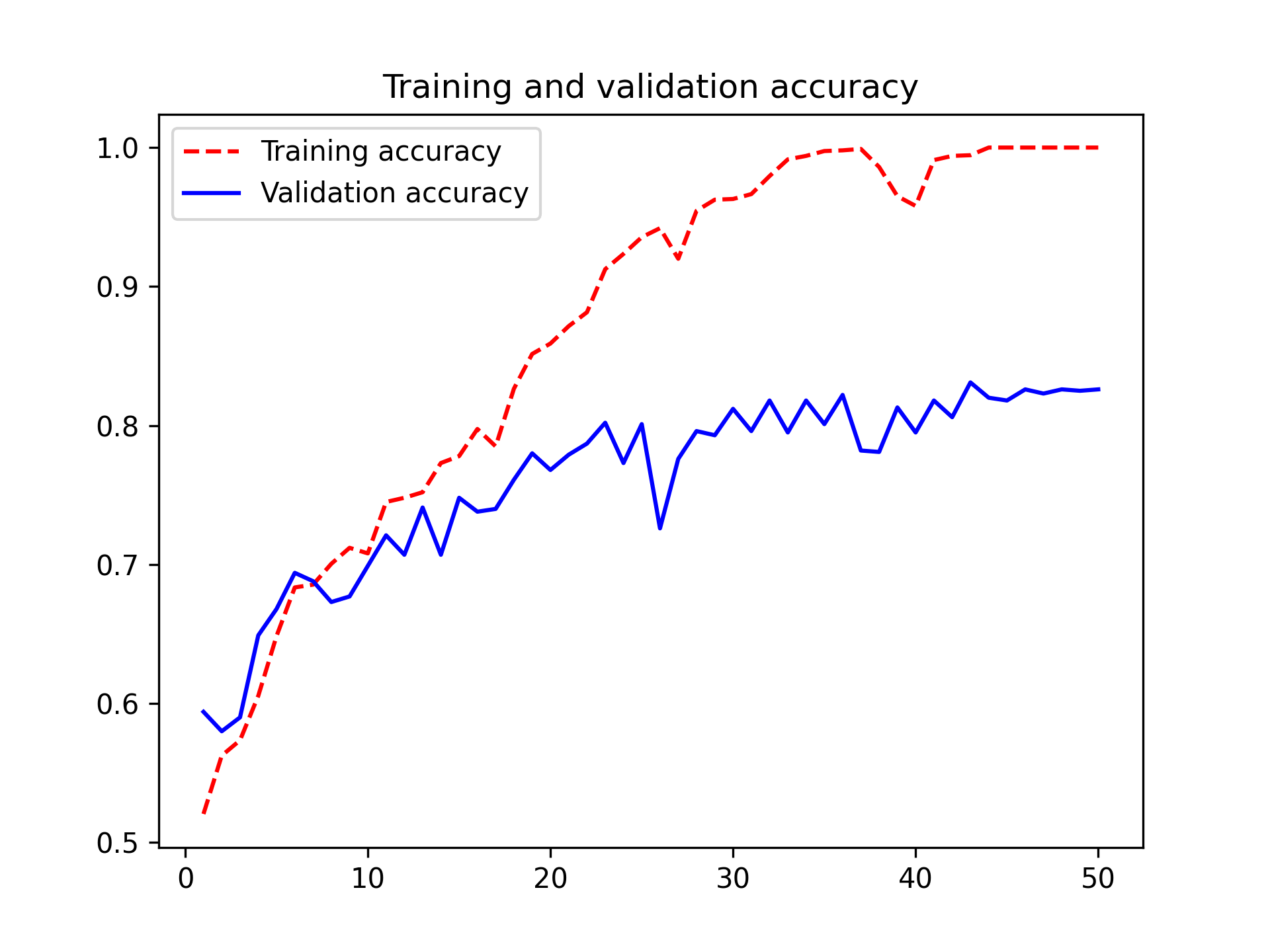
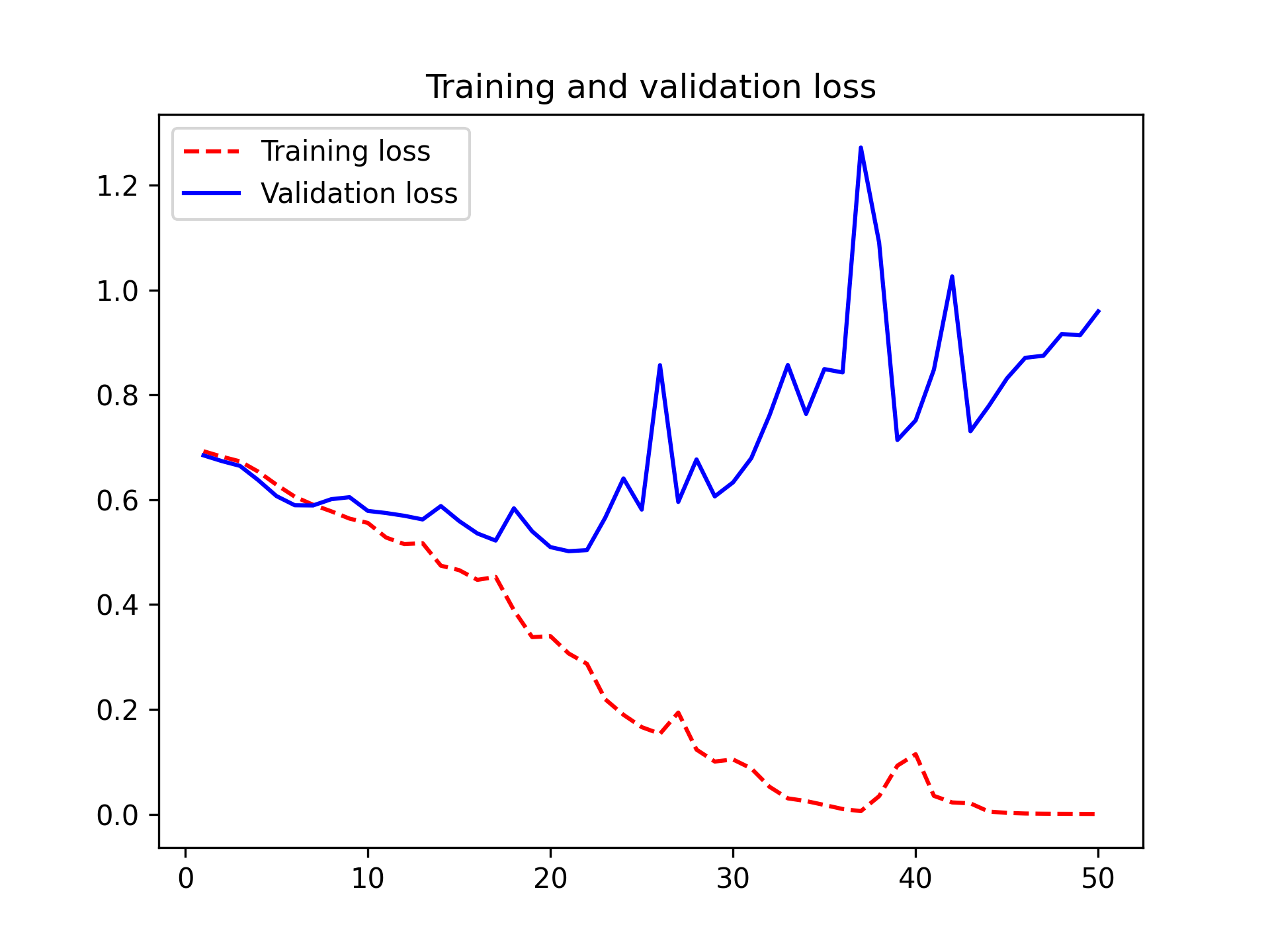
These plots are characteristic of overfitting. The training accuracy increases linearly over time, until it reaches nearly 100%, whereas the validation accuracy peaks around 80%. The validation loss reaches its minimum after only 10 epochs and then stalls, whereas the training loss keeps decreasing linearly as training proceeds.

Let's check the test accuracy. We'll reload the model from its saved file to evaluate it as it was before it started overfitting.

test_model = keras.models.load_model("convnet_from_scratch.keras")
test_loss, test_acc = test_model.evaluate(test_dataset)
print(f"Test accuracy: {test_acc:.3f}")

We get a test accuracy of 78.6% (due to the randomness of neural network initializations, you may get numbers within a few percentage points of that).

Because you have relatively few training samples (2,000), overfitting will be your number-one concern. You already know about a number of techniques that can help mitigate overfitting, such as dropout and weight decay (L2 regularization). We're now going to work with a new one, specific to computer vision and used almost universally when processing images with deep learning models: data augmentation.

Using data augmentation

Overfitting is caused by having too few samples to learn from, rendering you unable to train a model that can generalize to new data. Given infinite data, your model would be exposed to every possible aspect of the data distribution at hand: you would never overfit. Data augmentation takes the approach of generating more training data from existing training samples, by augmenting the samples via a number of random transformations that yield believable-looking images. The goal is that at training time, your model will never see the exact same picture twice. This helps expose the model to more aspects of the data and generalize better.

In Keras, this can be done via data augmentation layers. Such layers could be added in one of two ways:

• At the start of the model — Inside the model. In our case, the layers would come right before the Rescaling layer.
• Inside the data pipeline — Outside the model. In our case, we'd apply them to our Dataset via a map() call.

The main difference between these two options is that data augmentation done inside the model would be running on the GPU, just like the rest of the model. Meanwhile, data augmentation done in the data pipeline would be running on the CPU, typically in a parallel way on multiple CPU cores. Sometimes, there can be performance benefits to doing the former, but the latter is usually the better option. So let's go with that!

# Defines the transformations to apply as a list
data_augmentation_layers = [
    layers.RandomFlip("horizontal"),
    layers.RandomRotation(0.1),
    layers.RandomZoom(0.2),
]

# Creates a function that applies them sequentially
def data_augmentation(images, targets):
    for layer in data_augmentation_layers:
        images = layer(images)
    return images, targets

# Maps this function into the dataset
augmented_train_dataset = train_dataset.map(
    data_augmentation, num_parallel_calls=8
)
# Enables prefetching of batches on GPU memory; important for best
# performance
augmented_train_dataset = augmented_train_dataset.prefetch(tf.data.AUTOTUNE)

These are just a few of the layers available (for more, see the Keras documentation). Let's quickly go over this code:

• RandomFlip("horizontal") will apply horizontal flipping to a random 50% of the images that go through it.
• RandomRotation(0.1) will rotate the input images by a random value in the range [-10%, +10%] (these are fractions of a full circle — in degrees the range would be [-36 degrees, +36 degrees]).
• RandomZoom(0.2) will zoom in or out of the image by a random factor in the range [-20%, +20%].

Let's look at the augmented images (see figure 8.10).

plt.figure(figsize=(10, 10))
# You can use take(N) to only sample N batches from the dataset. This
# is equivalent to inserting a break in the loop after the Nth batch.
for image_batch, _ in train_dataset.take(1):
    image = image_batch[0]
    for i in range(9):
        ax = plt.subplot(3, 3, i + 1)
        augmented_image, _ = data_augmentation(image, None)
        augmented_image = keras.ops.convert_to_numpy(augmented_image)
        # Displays the first image in the output batch. For each of the
        # nine iterations, this is a different augmentation of the same
        # image.
        plt.imshow(augmented_image.astype("uint8"))
        plt.axis("off")

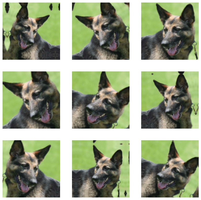
If you train a new model using this data-augmentation configuration, the model will never see the same input twice. But the inputs it sees are still heavily intercorrelated, because they come from a small number of original images — you can't produce new information; you can only remix existing information. As such, this may not be enough to completely get rid of overfitting. To further fight overfitting, you'll also add a Dropout layer to your model, right before the densely connected classifier.

inputs = keras.Input(shape=(180, 180, 3))
x = layers.Rescaling(1.0 / 255)(inputs)
x = layers.Conv2D(filters=32, kernel_size=3, activation="relu")(x)
x = layers.MaxPooling2D(pool_size=2)(x)
x = layers.Conv2D(filters=64, kernel_size=3, activation="relu")(x)
x = layers.MaxPooling2D(pool_size=2)(x)
x = layers.Conv2D(filters=128, kernel_size=3, activation="relu")(x)
x = layers.MaxPooling2D(pool_size=2)(x)
x = layers.Conv2D(filters=256, kernel_size=3, activation="relu")(x)
x = layers.MaxPooling2D(pool_size=2)(x)
x = layers.Conv2D(filters=512, kernel_size=3, activation="relu")(x)
x = layers.GlobalAveragePooling2D()(x)
x = layers.Dropout(0.25)(x)
outputs = layers.Dense(1, activation="sigmoid")(x)
model = keras.Model(inputs=inputs, outputs=outputs)

model.compile(
    loss="binary_crossentropy",
    optimizer="adam",
    metrics=["accuracy"],
)

Let's train the model using data augmentation and dropout. Because we expect overfitting to occur much later during training, we will train for twice as many epochs — 100. Note that we evaluate on images that aren't augmented — data augmentation is usually only performed at training time, as it is a regularization technique.

callbacks = [
    keras.callbacks.ModelCheckpoint(
        filepath="convnet_from_scratch_with_augmentation.keras",
        save_best_only=True,
        monitor="val_loss",
    )
]
history = model.fit(
    augmented_train_dataset,
    # Since we expect the model to overfit slower, we train for more
    # epochs.
    epochs=100,
    validation_data=validation_dataset,
    callbacks=callbacks,
)

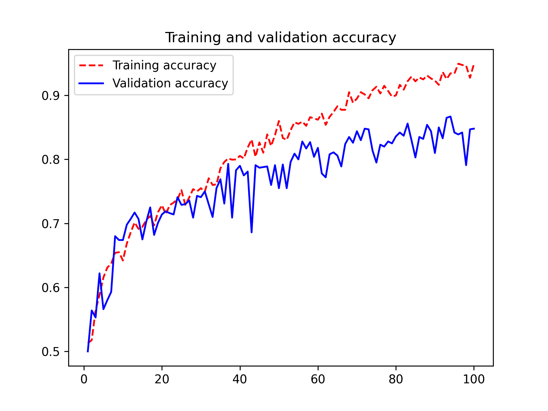
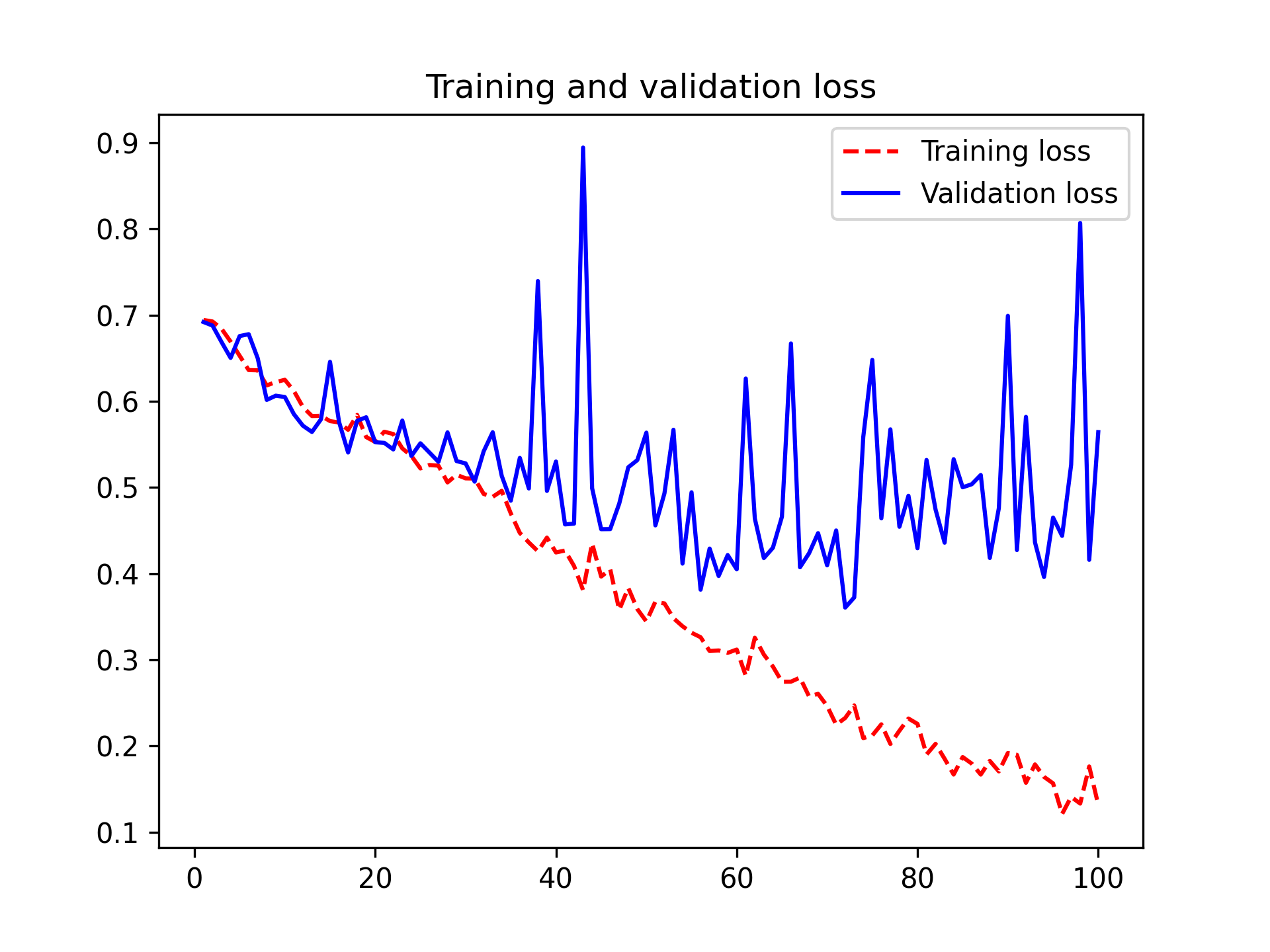
Let's plot the results again; see figure 8.11. Thanks to data augmentation and dropout, we start overfitting much later, around epochs 60-70 (compared to epoch 10 for the original model). The validation accuracy ends up peaking above 85% — a big improvement over our first try.

Let's check the test accuracy.

test_model = keras.models.load_model(
    "convnet_from_scratch_with_augmentation.keras"
)
test_loss, test_acc = test_model.evaluate(test_dataset)
print(f"Test accuracy: {test_acc:.3f}")

We get a test accuracy of 83.9%. It's starting to look good! If you're using Colab, make sure to download the saved file (convnet_from_scratch_with_augmentation.keras), as we will use it for some experiments in the next chapter.

By further tuning the model's configuration (such as the number of filters per convolution layer or the number of layers in the model), you may be able to get an even better accuracy, likely up to 90%. But it would prove difficult to go any higher just by training your own convnet from scratch because you have so little data to work with. As a next step to improve your accuracy on this problem, you'll have to use a pretrained model, which is the focus of the next two sections.

Using a pretrained model

A common and highly effective approach to deep learning on small image datasets is to use a pretrained model. A pretrained model is a model that was previously trained on a large dataset, typically on a large-scale image-classification task. If this original dataset is large enough and general enough, then the spatial hierarchy of features learned by the pretrained model can effectively act as a generic model of the visual world, and hence its features can prove useful for many different computer vision problems, even though these new problems may involve completely different classes than those of the original task. For instance, you might train a model on ImageNet (where classes are mostly animals and everyday objects) and then repurpose this trained model for something as remote as identifying furniture items in images. Such portability of learned features across different problems is a key advantage of deep learning compared to many older, shallow learning approaches, and it makes deep learning very effective for small-data problems.

In this case, let's consider a large convnet trained on the ImageNet dataset (1.4 million labeled images and 1,000 different classes). ImageNet contains many animal classes, including different species of cats and dogs, and you can thus expect it to perform well on the dogs-versus-cats classification problem.

We'll use the Xception architecture. This may be your first encounter with one of these cutesy model names — Xception, ResNet, EfficientNet, and so on; you'll get used to them if you keep doing deep learning for computer vision because they will come up frequently. You'll learn about the architectural details of Xception in the next chapter.

There are two ways to use a pretrained model: feature extraction and fine-tuning. We'll cover both of them. Let's start with feature extraction.

Feature extraction with a pretrained model

Feature extraction consists of using the representations learned by a previously trained model to extract interesting features from new samples. These features are then run through a new classifier, which is trained from scratch.

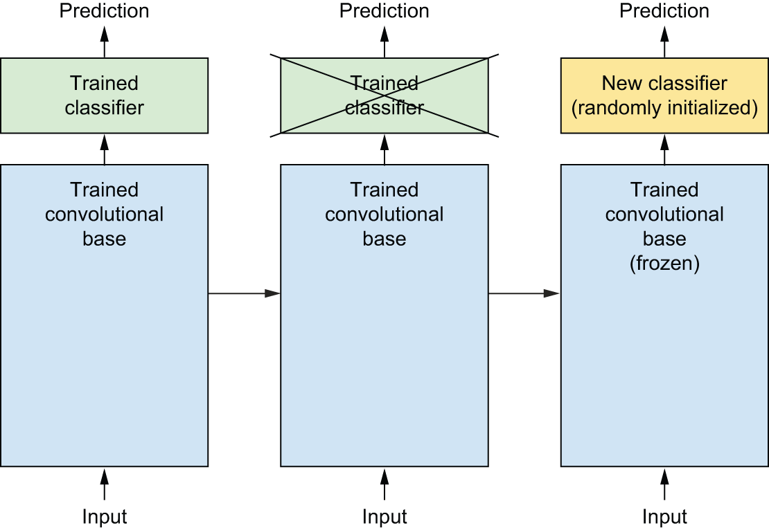
As you saw previously, convnets used for image classification comprise two parts: they start with a series of pooling and convolution layers, and they end with a densely connected classifier. The first part is called the convolutional base or backbone of the model. In the case of convnets, feature extraction consists of taking the convolutional base of a previously trained network, running the new data through it, and training a new classifier on top of the output (see figure 8.12).

Why only reuse the convolutional base? Could you reuse the densely connected classifier as well? In general, doing so should be avoided. The reason is that the representations learned by the convolutional base are likely to be more generic and therefore more reusable: the feature maps of a convnet are presence maps of generic concepts over a picture, which is likely to be useful regardless of the computer vision problem at hand. But the representations learned by the classifier will necessarily be specific to the set of classes on which the model was trained — they will only contain information about the presence probability of this or that class in the entire picture. Additionally, representations found in densely connected layers no longer contain any information about where objects are located in the input image: these layers get rid of the notion of space, whereas the object location is still described by convolutional feature maps. For problems where object location matters, densely connected features are largely useless.

Note that the level of generality (and therefore reusability) of the representations extracted by specific convolution layers depends on the depth of the layer in the model. Layers that come earlier in the model extract local, highly generic feature maps (such as visual edges, colors, and textures), whereas layers that are higher up extract more-abstract concepts (such as "cat ear" or "dog eye"). So if your new dataset differs a lot from the dataset on which the original model was trained, you may be better off using only the first few layers of the model to do feature extraction, rather than using the entire convolutional base.

In this case, because the ImageNet class set contains multiple dog and cat classes, it's likely to be beneficial to reuse the information contained in the densely connected layers of the original model. But we'll choose not to, so we can cover the more general case where the class set of the new problem doesn't overlap the class set of the original model. Let's put this in practice by using the convolutional base of our pretrained model to extract interesting features from cat and dog images and then train a dogs-versus-cats classifier on top of these features.

We will use the KerasHub library to create all pretrained models used in this book. KerasHub contains Keras implementations of popular pretrained model architectures paired with pretrained weights that can be downloaded to your machine. It contains a number of convnets like Xception, ResNet, EfficientNet and MobileNet, as well as larger, generative models we will use in the later chapters of this book. Let's try using it to instantiate the Xception model trained on the ImageNet dataset.

import keras_hub

conv_base = keras_hub.models.Backbone.from_preset("xception_41_imagenet")

You'll note a couple of things. First, KerasHub uses the term backbone to refer to the underlying feature extractor network without the classification head (it's a little easier to type than "convolutional base"). It also uses a special constructor called from_preset() that will download the configuration and weights for the Xception model.

What's that "41" in the name of the model we are using? Pretrained convnets are by convention often named by how "deep" they are. In this case, the 41 means that our Xception model has 41 trainable layers (conv and dense layers) stacked on top of each other. It's the "deepest" model we've used so far in the book by a good margin.

There's one more missing piece we need before we can use this model. Every pretrained convnet will do some rescaling and resizing of images before pretraining. It's important to make sure our input images match; otherwise, our model will need to relearn how to extract features from images with a totally different input range. Rather than keep track of which pretrained models use a [0, 1] input range for pixel values and which use a [-1, 1] range, we can use a KerasHub layer called ImageConverter that will rescale our images to match our pretrained checkpoint. It has the same special from_preset() constructor as the backbone class.

preprocessor = keras_hub.layers.ImageConverter.from_preset(
    "xception_41_imagenet",
    image_size=(180, 180),
)

At this point, there are two ways you could proceed:

• Running the convolutional base over your dataset, recording its output to a NumPy array on disk, and then using this data as input to a standalone, densely connected classifier similar to those you saw in part 1 of this book. This solution is fast and cheap to run, because it only requires running the convolutional base once for every input image, and the convolutional base is by far the most expensive part of the pipeline. But for the same reason, this technique won't allow you to use data augmentation.

• Extending the model you have (conv_base) by adding Dense layers on top and running the whole thing end to end on the input data. This will allow you to use data augmentation because every input image goes through the convolutional base every time it's seen by the model. But for the same reason, this technique is far more expensive than the first.

We'll cover both techniques. Let's walk through the code required to set up the first one: recording the output of conv_base on your data and using these outputs as inputs to a new model.

Fast feature extraction without data augmentation

You'll start by extracting features as NumPy arrays, by calling the predict() method of the conv_base model on our training, validation, and testing datasets. Let's iterate over our datasets to extract the pretrained model's features.

def get_features_and_labels(dataset):
    all_features = []
    all_labels = []
    for images, labels in dataset:
        preprocessed_images = preprocessor(images)
        features = conv_base.predict(preprocessed_images, verbose=0)
        all_features.append(features)
        all_labels.append(labels)
    return np.concatenate(all_features), np.concatenate(all_labels)

train_features, train_labels = get_features_and_labels(train_dataset)
val_features, val_labels = get_features_and_labels(validation_dataset)
test_features, test_labels = get_features_and_labels(test_dataset)

Importantly, predict() only expects images, not labels, but our current dataset yields batches that contain both images and their labels.

The extracted features are currently of shape (samples, 6, 6, 2048):

>>> train_features.shape
(2000, 6, 6, 2048)

At this point, you can define your densely connected classifier (note the use of dropout for regularization) and train it on the data and labels that you just recorded.

inputs = keras.Input(shape=(6, 6, 2048))
# Averages spatial dimensions to flatten the feature map.
x = layers.GlobalAveragePooling2D()(inputs)
x = layers.Dense(256, activation="relu")(x)
x = layers.Dropout(0.25)(x)
outputs = layers.Dense(1, activation="sigmoid")(x)
model = keras.Model(inputs, outputs)
model.compile(
    loss="binary_crossentropy",
    optimizer="adam",
    metrics=["accuracy"],
)

callbacks = [
    keras.callbacks.ModelCheckpoint(
        filepath="feature_extraction.keras",
        save_best_only=True,
        monitor="val_loss",
    )
]
history = model.fit(
    train_features,
    train_labels,
    epochs=10,
    validation_data=(val_features, val_labels),
    callbacks=callbacks,
)

Training is very fast because you only have to deal with two Dense layers — an epoch takes less than 1 second even on CPU.

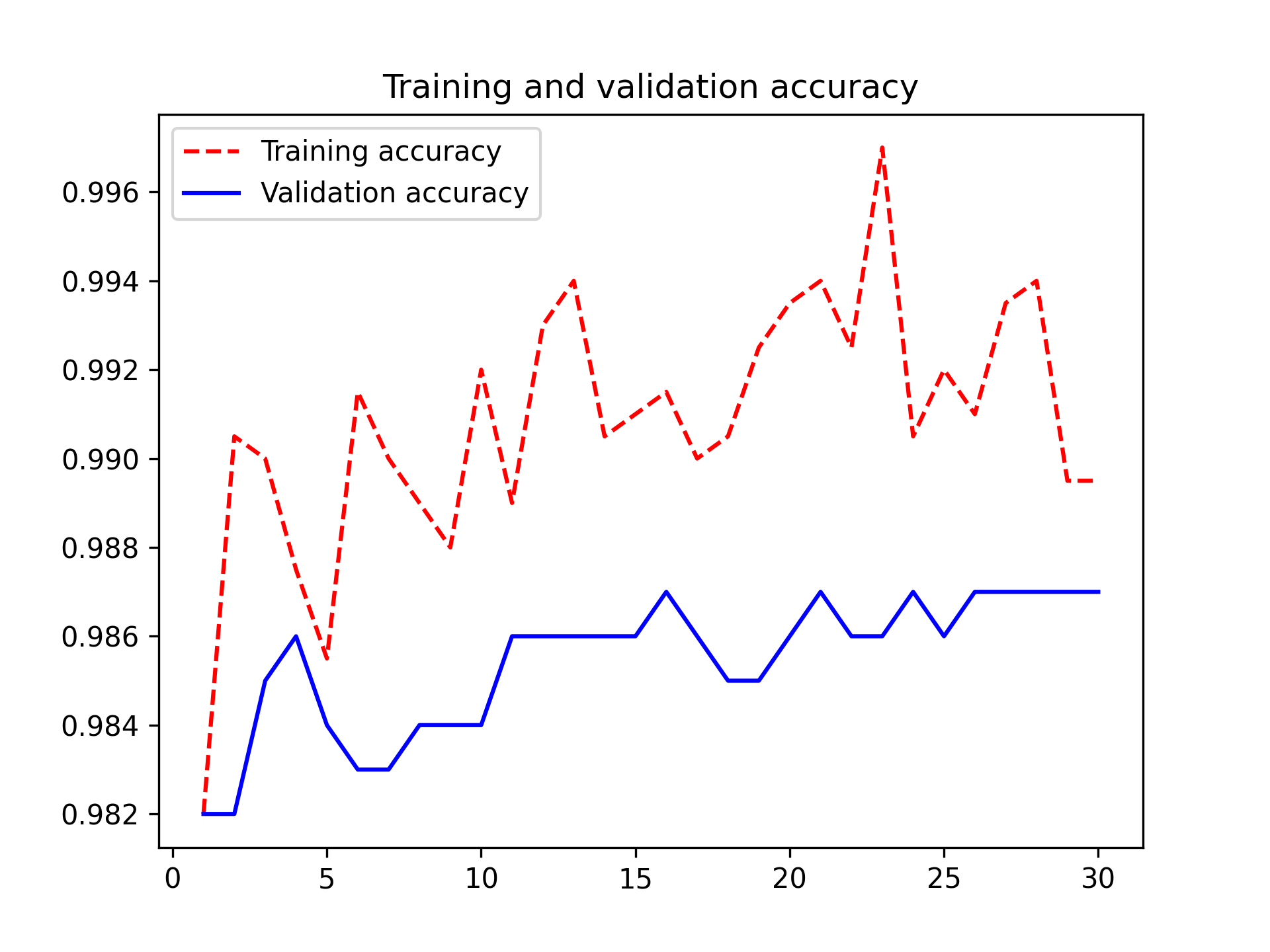
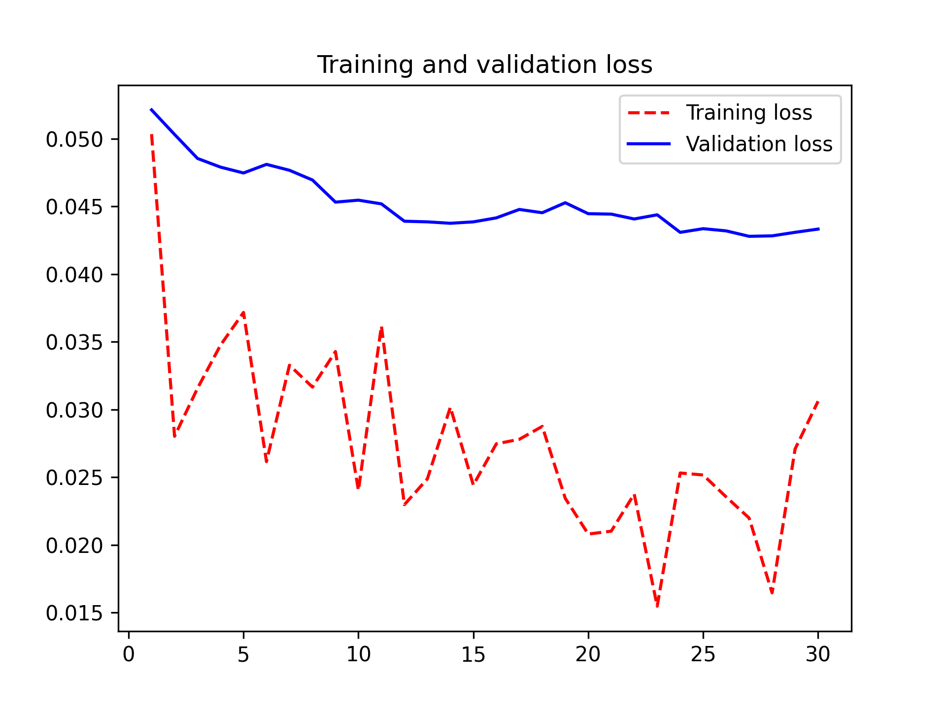
Let's look at the loss and accuracy curves during training (see figure 8.13).

import matplotlib.pyplot as plt

acc = history.history["accuracy"]
val_acc = history.history["val_accuracy"]
loss = history.history["loss"]
val_loss = history.history["val_loss"]
epochs = range(1, len(acc) + 1)
plt.plot(epochs, acc, "r--", label="Training accuracy")
plt.plot(epochs, val_acc, "b", label="Validation accuracy")
plt.title("Training and validation accuracy")
plt.legend()
plt.figure()
plt.plot(epochs, loss, "r--", label="Training loss")
plt.plot(epochs, val_loss, "b", label="Validation loss")
plt.title("Training and validation loss")
plt.legend()
plt.show()

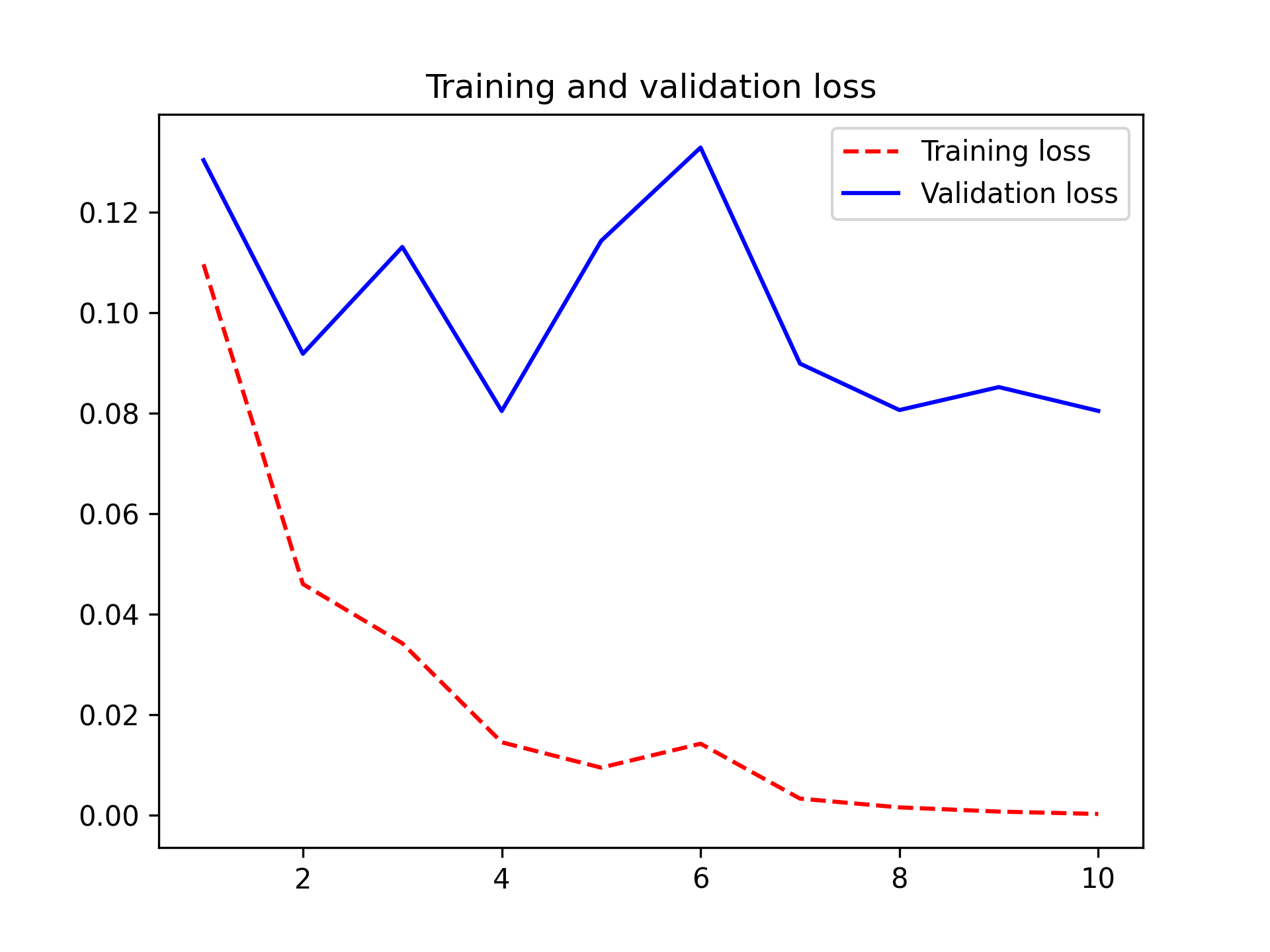
You reach a validation accuracy of slightly over 98% — much better than you achieved in the previous section with the small model trained from scratch. This is a bit of an unfair comparison, however, because ImageNet contains many dogs and cats instances, which means that our pretrained model already has the exact knowledge required for the task at hand. This won't always be the case when you use pretrained features.

However, the plots also indicate that you're overfitting almost from the start — despite using dropout with a fairly large rate. That's because this technique doesn't use data augmentation, which is essential for preventing overfitting with small image datasets.

Let's check the test accuracy:

test_model = keras.models.load_model("feature_extraction.keras")
test_loss, test_acc = test_model.evaluate(test_features, test_labels)
print(f"Test accuracy: {test_acc:.3f}")

We get test accuracy of 98.1% — a very nice improvement over training a model from scratch!

Feature extraction together with data augmentation

Now, let's review the second technique we mentioned for doing feature extraction, which is much slower and more expensive but allows you to use data augmentation during training: creating a model that chains the conv_base with a new dense classifier and training it end to end on the inputs.

To do this, we will first freeze the convolutional base. Freezing a layer or set of layers means preventing their weights from being updated during training. Here, if you don't do this, then the representations that were previously learned by the convolutional base will be modified during training. Because the Dense layers on top are randomly initialized, very large weight updates would be propagated through the network, effectively destroying the representations previously learned.

In Keras, you freeze a layer or model by setting its trainable attribute to False.

import keras_hub

conv_base = keras_hub.models.Backbone.from_preset(
    "xception_41_imagenet",
    trainable=False,
)

Setting trainable to False empties the list of trainable weights of the layer or model.

>>> conv_base.trainable = True
>>> # The number of trainable weights before freezing the conv base
>>> len(conv_base.trainable_weights)
154
>>> conv_base.trainable = False
>>> # The number of trainable weights after freezing the conv base
>>> len(conv_base.trainable_weights)
0

Now, we can just create a new model that chains together our frozen convolutional base and a dense classifier, like this:

inputs = keras.Input(shape=(180, 180, 3))
x = preprocessor(inputs)
x = conv_base(x)
x = layers.GlobalAveragePooling2D()(x)
x = layers.Dense(256)(x)
x = layers.Dropout(0.25)(x)
outputs = layers.Dense(1, activation="sigmoid")(x)
model = keras.Model(inputs, outputs)
model.compile(
    loss="binary_crossentropy",
    optimizer="adam",
    metrics=["accuracy"],
)

With this setup, only the weights from the two Dense layers that you added will be trained. That's a total of four weight tensors: two per layer (the main weight matrix and the bias vector). Note that for these changes to take effect, you must first compile the model. If you ever modify weight trainability after compilation, you should then recompile the model, or these changes will be ignored.

Let's train our model. We'll reuse our augmented dataset augmented_train_dataset. Thanks to data augmentation, it will take much longer for the model to start overfitting, so we can train for more epochs — let's do 30:

callbacks = [
    keras.callbacks.ModelCheckpoint(
        filepath="feature_extraction_with_data_augmentation.keras",
        save_best_only=True,
        monitor="val_loss",
    )
]
history = model.fit(
    augmented_train_dataset,
    epochs=30,
    validation_data=validation_dataset,
    callbacks=callbacks,
)

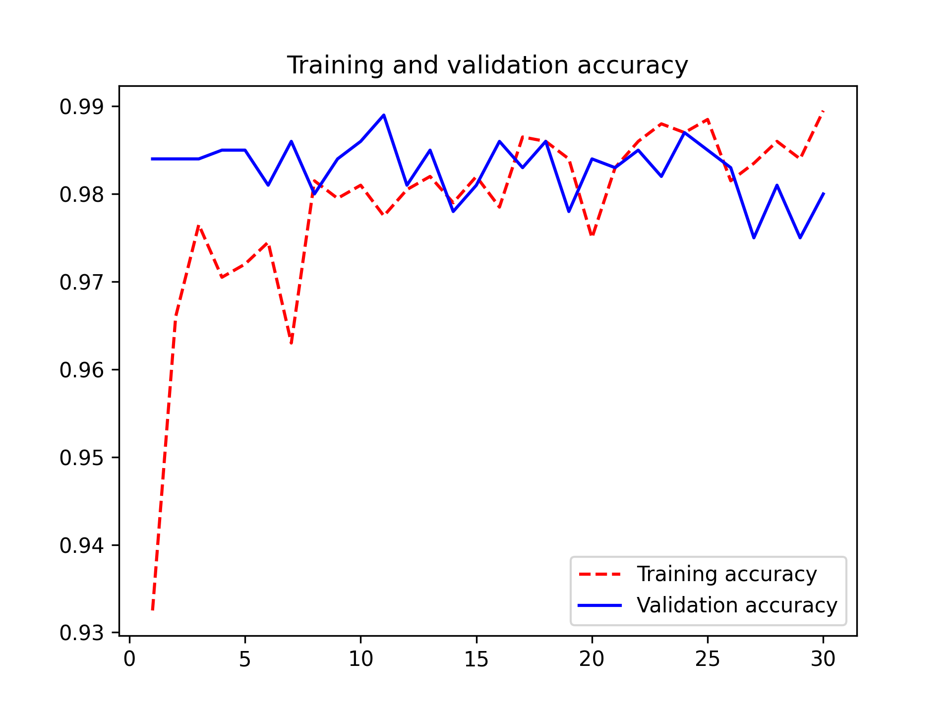
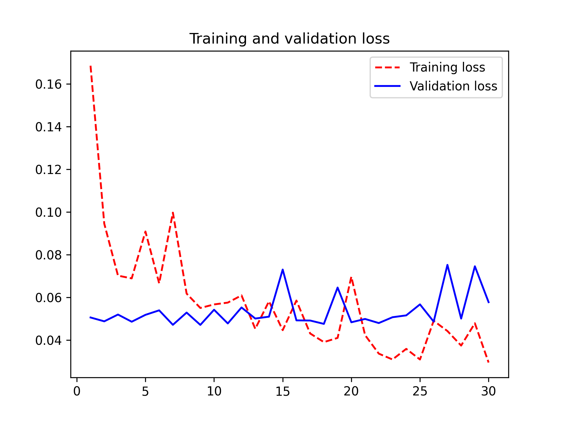
Let's plot the results again (see figure 8.14). This model reaches a validation accuracy of 98.2%.

Let's check the test accuracy.

test_model = keras.models.load_model(
    "feature_extraction_with_data_augmentation.keras"
)
test_loss, test_acc = test_model.evaluate(test_dataset)
print(f"Test accuracy: {test_acc:.3f}")

We get a test accuracy of 98.4%. This is not an improvement over the previous model, which is a bit disappointing. This could be a sign that our data augmentation configuration does not exactly match the distribution of the test data. Let's see if we can do better with our latest attempt.

Fine-tuning a pretrained model

Another widely used technique for model reuse, complementary to feature extraction, is fine-tuning (see figure 8.15). Fine-tuning consists of unfreezing the frozen model base used for feature extraction and jointly training both the newly added part of the model (in this case, the fully connected classifier) and the base model. This is called fine-tuning because it slightly adjusts the more abstract representations of the model being reused to make them more relevant for the problem at hand.

We stated earlier that it's necessary to freeze the pretrained convolution base first to be able to train a randomly initialized classifier on top. For the same reason, it's only possible to fine-tune the convolutional base once the classifier on top has already been trained. If the classifier isn't already trained, then the error signal propagating through the network during training will be too large, and the representations previously learned by the layers being fine-tuned will be destroyed. Thus, the steps for fine-tuning a network are as follows:

1. Add your custom network on top of an already-trained base network.
2. Freeze the base network.
3. Train the part you added.
4. Unfreeze the base network.
5. Jointly train both these layers and the part you added.

Note that you should not unfreeze "batch normalization" layers (BatchNormalization). Batch normalization and its effect on fine-tuning is explained in the next chapter.

You already completed the first three steps when doing feature extraction. Let's proceed with step 4: you'll unfreeze your conv_base.

Let's start fine-tuning the model using a very low learning rate. The reason for using a low learning rate is that you want to limit the magnitude of the modifications you make to the representations of the layers you're fine-tuning. Updates that are too large may harm these representations.

model.compile(
    loss="binary_crossentropy",
    optimizer=keras.optimizers.Adam(learning_rate=1e-5),
    metrics=["accuracy"],
)

callbacks = [
    keras.callbacks.ModelCheckpoint(
        filepath="fine_tuning.keras",
        save_best_only=True,
        monitor="val_loss",
    )
]
history = model.fit(
    augmented_train_dataset,
    epochs=30,
    validation_data=validation_dataset,
    callbacks=callbacks,
)

You can now finally evaluate this model on the test data (see figure 8.15):

model = keras.models.load_model("fine_tuning.keras")
test_loss, test_acc = model.evaluate(test_dataset)
print(f"Test accuracy: {test_acc:.3f}")

Here, you get a test accuracy of 98.6% (again, your own results may be within half a percentage point). In the original Kaggle competition around this dataset, this would have been one of the top results. It's not quite a fair comparison, however, since you used pretrained features that already contained prior knowledge about cats and dogs, which competitors couldn't use at the time.

On the positive side, by using modern deep learning techniques, you managed to reach this result using only a small fraction of the training data that was available for the competition (about 10%). There is a huge difference between being able to train on 20,000 samples compared to 2,000 samples!

Now you have a solid set of tools for dealing with image-classification problems — in particular, with small datasets.

Summary

• Convnets excel at computer vision tasks. It's possible to train one from scratch, even on a very small dataset, with decent results.
• Convnets work by learning a hierarchy of modular patterns and concepts to represent the visual world.
• On a small dataset, overfitting will be the main issue. Data augmentation is a powerful way to fight overfitting when you're working with image data.
• It's easy to reuse an existing convnet on a new dataset via feature extraction. This is a valuable technique for working with small image datasets.
• As a complement to feature extraction, you can use fine-tuning, which adapts to a new problem some of the representations previously learned by an existing model. This pushes performance a bit further.