


A fundamental problem when building a computer vision application is that of interpretability: Why did your classifier think a particular image contained a fridge, when all you can see is a truck? This is especially relevant to use cases where deep learning is used to complement human expertise, such as medical imaging use cases. This chapter will get you familiar with a range of different techniques for visualizing what ConvNets learn and understanding the decisions they make.
It’s often said that deep learning models are “black boxes”: they learn representations that are difficult to extract and present in a human-readable form. Although this is partially true for certain types of deep learning models, it’s definitely not true for ConvNets. The representations learned by ConvNets are highly amenable to visualization, in large part because they’re representations of visual concepts. Since 2013, a wide array of techniques has been developed for visualizing and interpreting these representations. We won’t survey all of them, but we’ll cover three of the most accessible and useful ones:
- Visualizing intermediate ConvNet outputs (intermediate activations) — Useful for understanding how successive ConvNet layers transform their input, and for getting a first idea of the meaning of individual ConvNet filters
- Visualizing ConvNets filters — Useful for understanding precisely what visual pattern or concept each filter in a ConvNet is receptive to
- Visualizing heatmaps of class activation in an image — Useful for understanding which parts of an image were identified as belonging to a given class, thus allowing you to localize objects in images
For the first method — activation visualization — you’ll use the small ConvNet that you trained from scratch on the dogs-versus-cats classification problem in chapter 8. For the next two methods, you’ll use a pretrained Xception model.
Visualizing intermediate activations
Visualizing intermediate activations consists of displaying the values returned by various convolution and pooling layers in a model, given a certain input (the output of a layer is often called its activation, the output of the activation function). This gives a view into how an input is decomposed into the different filters learned by the network. You want to visualize feature maps with three dimensions: width, height, and depth (channels). Each channel encodes relatively independent features, so the proper way to visualize these feature maps is by independently plotting the contents of every channel as a 2D image. Let’s start by loading the model that you saved in section 8.2:
>>> import keras >>> model = keras.models.load_model( ... "convnet_from_scratch_with_augmentation.keras" ... ) >>> model.summary()Model: "functional_3" ┏━━━━━━━━━━━━━━━━━━━━━━━━━━━━━━━━━━━┳━━━━━━━━━━━━━━━━━━━━━━━━━━┳━━━━━━━━━━━━━━━┓ ┃ Layer (type) ┃ Output Shape ┃ Param # ┃ ┡━━━━━━━━━━━━━━━━━━━━━━━━━━━━━━━━━━━╇━━━━━━━━━━━━━━━━━━━━━━━━━━╇━━━━━━━━━━━━━━━┩ │ input_layer_3 (InputLayer) │ (None, 180, 180, 3) │ 0 │ ├───────────────────────────────────┼──────────────────────────┼───────────────┤ │ rescaling_1 (Rescaling) │ (None, 180, 180, 3) │ 0 │ ├───────────────────────────────────┼──────────────────────────┼───────────────┤ │ conv2d_11 (Conv2D) │ (None, 178, 178, 32) │ 896 │ ├───────────────────────────────────┼──────────────────────────┼───────────────┤ │ max_pooling2d_6 (MaxPooling2D) │ (None, 89, 89, 32) │ 0 │ ├───────────────────────────────────┼──────────────────────────┼───────────────┤ │ conv2d_12 (Conv2D) │ (None, 87, 87, 64) │ 18,496 │ ├───────────────────────────────────┼──────────────────────────┼───────────────┤ │ max_pooling2d_7 (MaxPooling2D) │ (None, 43, 43, 64) │ 0 │ ├───────────────────────────────────┼──────────────────────────┼───────────────┤ │ conv2d_13 (Conv2D) │ (None, 41, 41, 128) │ 73,856 │ ├───────────────────────────────────┼──────────────────────────┼───────────────┤ │ max_pooling2d_8 (MaxPooling2D) │ (None, 20, 20, 128) │ 0 │ ├───────────────────────────────────┼──────────────────────────┼───────────────┤ │ conv2d_14 (Conv2D) │ (None, 18, 18, 256) │ 295,168 │ ├───────────────────────────────────┼──────────────────────────┼───────────────┤ │ max_pooling2d_9 (MaxPooling2D) │ (None, 9, 9, 256) │ 0 │ ├───────────────────────────────────┼──────────────────────────┼───────────────┤ │ conv2d_15 (Conv2D) │ (None, 7, 7, 512) │ 1,180,160 │ ├───────────────────────────────────┼──────────────────────────┼───────────────┤ │ global_average_pooling2d_3 │ (None, 512) │ 0 │ │ (GlobalAveragePooling2D) │ │ │ ├───────────────────────────────────┼──────────────────────────┼───────────────┤ │ dropout (Dropout) │ (None, 512) │ 0 │ ├───────────────────────────────────┼──────────────────────────┼───────────────┤ │ dense_3 (Dense) │ (None, 1) │ 513 │ └───────────────────────────────────┴──────────────────────────┴───────────────┘ Total params: 4,707,269 (17.96 MB) Trainable params: 1,569,089 (5.99 MB) Non-trainable params: 0 (0.00 B) Optimizer params: 3,138,180 (11.97 MB)
Next, you’ll get an input image — a picture of a cat, not part of the images the network was trained on.
import keras
import numpy as np

# Downloads a test image
img_path = keras.utils.get_file(
    fname="cat.jpg", origin="https://img-datasets.s3.amazonaws.com/cat.jpg"
)

def get_img_array(img_path, target_size):
    # Opens the image file and resizes it
    img = keras.utils.load_img(img_path, target_size=target_size)
    # Turns the image into a float32 NumPy array of shape (180, 180, 3)
    array = keras.utils.img_to_array(img)
    # We add a dimension to transform our array into a "batch" of a
    # single sample. Its shape is now (1, 180, 180, 3).
    array = np.expand_dims(array, axis=0)
    return array

img_tensor = get_img_array(img_path, target_size=(180, 180))
Let’s display the picture (see figure 10.1).
import matplotlib.pyplot as plt

plt.axis("off")
plt.imshow(img_tensor[0].astype("uint8"))
plt.show()

To extract the feature maps you want to look at, you’ll create a Keras model that takes batches of images as input and outputs the activations of all convolution and pooling layers.
from keras import layers

layer_outputs = []
layer_names = []
# Extracts the outputs of all Conv2D and MaxPooling2D layers and put
# them in a list
for layer in model.layers:
    if isinstance(layer, (layers.Conv2D, layers.MaxPooling2D)):
        layer_outputs.append(layer.output)
        # Saves the layer names for later
        layer_names.append(layer.name)
# Creates a model that will return these outputs, given the model input
activation_model = keras.Model(inputs=model.input, outputs=layer_outputs)
When fed an image input, this model returns the values of the layer activations in the original model, as a list. This is the first time you’ve encountered a multi-output model in this book in practice since you learned about them in chapter 7: until now, the models you’ve seen have had exactly one input and one output. This one has one input and nine outputs — one output per layer activation.
# Returns a list of nine NumPy arrays — one array per layer activation
activations = activation_model.predict(img_tensor)
For instance, this is the activation of the first convolution layer for the cat image input:
>>> first_layer_activation = activations[0] >>> print(first_layer_activation.shape)(1, 178, 178, 32)
It’s a 178 × 178 feature map with 32 channels. Let’s try plotting the sixth channel of the activation of the first layer of the original model (see figure 10.2).
import matplotlib.pyplot as plt

plt.matshow(first_layer_activation[0, :, :, 5], cmap="viridis")
This channel appears to encode a diagonal edge detector, but note that your own channels may vary because the specific filters learned by convolution layers aren’t deterministic.
Now let’s plot a complete visualization of all the activations in the network (see figure 10.3). We’ll extract and plot every channel in each of the layer activations, and we’ll stack the results in one big grid, with channels stacked side by side.
images_per_row = 16
# Iterates over the activations (and the names of the corresponding
# layers)
for layer_name, layer_activation in zip(layer_names, activations):
    # The layer activation has shape (1, size, size, n_features).
    n_features = layer_activation.shape[-1]
    size = layer_activation.shape[1]
    n_cols = n_features // images_per_row
    # Prepares an empty grid for displaying all the channels in this
    # activation
    display_grid = np.zeros(
        ((size + 1) * n_cols - 1, images_per_row * (size + 1) - 1)
    )
    for col in range(n_cols):
        for row in range(images_per_row):
            channel_index = col * images_per_row + row
            # This is a single channel (or feature).
            channel_image = layer_activation[0, :, :, channel_index].copy()
            # Normalizes channel values within the [0, 255] range.
            # All-zero channels are kept at zero.
            if channel_image.sum() != 0:
                channel_image -= channel_image.mean()
                channel_image /= channel_image.std()
                channel_image *= 64
                channel_image += 128
            channel_image = np.clip(channel_image, 0, 255).astype("uint8")
            # Places the channel matrix in the empty grid we prepared
            display_grid[
                col * (size + 1) : (col + 1) * size + col,
                row * (size + 1) : (row + 1) * size + row,
            ] = channel_image
    # Displays the grid for the layer
    scale = 1.0 / size
    plt.figure(
        figsize=(scale * display_grid.shape[1], scale * display_grid.shape[0])
    )
    plt.title(layer_name)
    plt.grid(False)
    plt.axis("off")
    plt.imshow(display_grid, aspect="auto", cmap="viridis")
There are a few things to note here:
- The first layer acts as a collection of various edge detectors. At that stage, the activations retain almost all of the information present in the initial picture.
- As you go higher, the activations become increasingly abstract and less visually interpretable. They begin to encode higher-level concepts such as “cat ear” and “cat eye.” Higher representations carry increasingly less information about the visual contents of the image and increasingly more information related to the class of the image.
- The sparsity of the activations increases with the depth of the layer: in the first layer, all filters are activated by the input image, but in the following layers, more and more filters are blank. This means the pattern encoded by the filter isn’t found in the input image.
We have just observed an important universal characteristic of the representations learned by deep neural networks: the features extracted by a layer become increasingly abstract with the depth of the layer. The activations of higher layers carry less and less information about the specific input being seen and more and more information about the target (in this case, the class of the image: cat or dog). A deep neural network effectively acts as an information distillation pipeline, with raw data going in (in this case, RGB pictures) and being repeatedly transformed so that irrelevant information is filtered out (for example, the specific visual appearance of the image) and useful information is magnified and refined (for example, the class of the image).
This is analogous to the way humans and animals perceive the world: after observing a scene for a few seconds, a human can remember which abstract objects were present in it (bicycle, tree) but can’t remember the specific appearance of these objects. In fact, if you tried to draw a generic bicycle from memory, chances are you couldn’t get it even remotely right, even though you’ve seen thousands of bicycles in your lifetime (see, for example, figure 10.4). Try it right now: this effect is absolutely real. Your brain has learned to completely abstract its visual input — to transform it into high-level visual concepts while filtering out irrelevant visual details — making it tremendously difficult to remember how things around you look.
Visualizing ConvNet filters
Another easy way to inspect the filters learned by ConvNets is to display the visual pattern that each filter is meant to respond to. This can be done with gradient ascent in input space, applying gradient descent to the value of the input image of a ConvNet so as to maximize the response of a specific filter, starting from a blank input image. The resulting input image will be one that the chosen filter is maximally responsive to.
Let’s try this with the filters of the Xception model. The process is simple: we’ll build a loss function that maximizes the value of a given filter in a given convolution layer, and then we’ll use stochastic gradient descent to adjust the values of the input image so as to maximize this activation value. This will be your second example of a low-level gradient descent loop (the first one was in chapter 2). We will show it for TensorFlow, PyTorch, and Jax.
First, let’s instantiate the Xception model trained on the ImageNet dataset. We can once again use the KerasHub library, exactly as we did in chapter 8.
import keras_hub

# Instantiates the feature extractor network from pretrained weights
model = keras_hub.models.Backbone.from_preset(
    "xception_41_imagenet",
)
# Loads the matching preprocessing to scale our input images
preprocessor = keras_hub.layers.ImageConverter.from_preset(
    "xception_41_imagenet",
    image_size=(180, 180),
)
We’re interested in the convolutional layers of the model — the Conv2D
and SeparableConv2D layers. We’ll need to know their names so we can
retrieve their outputs. Let’s print their names, in order of depth.
for layer in model.layers:
    if isinstance(layer, (keras.layers.Conv2D, keras.layers.SeparableConv2D)):
        print(layer.name)
You’ll notice that the SeparableConv2D layers here are all named something like
block6_sepconv1, block7_sepconv2, etc. — Xception is structured into blocks,
each containing several convolutional layers.
Now let’s create a second model that returns the output of a specific layer
— a “feature extractor” model.
Because our model is a Functional API model,
it is inspectable: you can query the output of one of its layers and reuse
it in a new model. No need to copy the entire Xception code.
# You could replace this with the name of any layer in the Xception
# convolutional base.
layer_name = "block3_sepconv1"
# This is the layer object we're interested in.
layer = model.get_layer(name=layer_name)
# We use model.input and layer.output to create a model that, given an
# input image, returns the output of our target layer.
feature_extractor = keras.Model(inputs=model.input, outputs=layer.output)
To use this model, we can simply call it on some input data, but we should be careful to apply our model-specific image preprocessing so that our images are scaled to the same range as the Xception pretraining data.
activation = feature_extractor(preprocessor(img_tensor))
Let’s use our feature extractor model to define a function that returns a scalar value quantifying how much a given input image “activates” a given filter in the layer. This is the loss function that we’ll maximize during the gradient ascent process:
from keras import ops

# The loss function takes an image tensor and the index of the filter
# we consider (an integer).
def compute_loss(image, filter_index):
    activation = feature_extractor(image)
    # We avoid border artifacts by only involving nonborder pixels in
    # the loss: we discard the first 2 pixels along the sides of the
    # activation.
    filter_activation = activation[:, 2:-2, 2:-2, filter_index]
    # Returns the mean of the activation values for the filter
    return ops.mean(filter_activation)
A non-obvious trick to help the gradient-ascent process go smoothly is to normalize the gradient tensor by dividing it by its L2 norm (the square root of the sum of the squares of the values in the tensor). This ensures that the magnitude of the updates done to the input image is always within the same range.
Let’s set up the gradient ascent step function. Anything that involves
gradients requires calling backend-level APIs, such as GradientTape in TensorFlow,
.backward() in PyTorch, and jax.grad() in JAX. Let’s line up all the code snippets for
each of the three backends, starting with TensorFlow.
Gradient ascent in TensorFlow
For TensorFlow, we can just open a GradientTape scope and compute the loss
inside of it to retrieve the gradients we need. We’ll use a @tf.function
decorator to speed up computation:
import tensorflow as tf

@tf.function
def gradient_ascent_step(image, filter_index, learning_rate):
    with tf.GradientTape() as tape:
        # Explicitly watches the image tensor, since it isn't a
        # TensorFlow Variable (only Variables are automatically watched
        # in a gradient tape)
        tape.watch(image)
        # Computes the loss scalar, indicating how much the current
        # image activates the filter
        loss = compute_loss(image, filter_index)
    # Computes the gradients of the loss with respect to the image
    grads = tape.gradient(loss, image)
    # Applies the "gradient normalization trick"
    grads = ops.normalize(grads)
    # Moves the image a little bit in a direction that activates our
    # target filter more strongly
    image += learning_rate * grads
    # Returns the updated image, so we can run the step function in a
    # loop
    return image
Gradient ascent in PyTorch
In the case of PyTorch, we use loss.backward() and image.grad to obtain
the gradients of the loss with respect to the input image, like this.
import torch

def gradient_ascent_step(image, filter_index, learning_rate):
    # Creates a copy of "image" that we can get gradients for.
    image = image.clone().detach().requires_grad_(True)
    loss = compute_loss(image, filter_index)
    loss.backward()
    grads = image.grad
    grads = ops.normalize(grads)
    image = image + learning_rate * grads
    return image
No need to reset the gradients since the image tensor is recreated at each iteration.
Gradient ascent in JAX
In the case of JAX, we use jax.grad() to obtain a function that returns the
gradients of the loss with respect to the input image.
import jax

grad_fn = jax.grad(compute_loss)

@jax.jit
def gradient_ascent_step(image, filter_index, learning_rate):
    grads = grad_fn(image, filter_index)
    grads = ops.normalize(grads)
    image += learning_rate * grads
    return image
The filter visualization loop
Now you have all the pieces. Let’s put them together into a Python function that takes a filter index as input and returns a tensor representing the pattern that maximizes the activation of the specified filter in our target layer.
img_width = 200
img_height = 200

def generate_filter_pattern(filter_index):
    # The number of gradient ascent steps to apply
    iterations = 30
    # The amplitude of a single step
    learning_rate = 10.0
    image = keras.random.uniform(
        # Initialize an image tensor with random values. (The Xception
        # model expects input values in the [0, 1] range, so here we
        # pick a range centered on 0.5.)
        minval=0.4, maxval=0.6, shape=(1, img_width, img_height, 3)
    )
    # Repeatedly updates the values of the image tensor to maximize our
    # loss function
    for i in range(iterations):
        image = gradient_ascent_step(image, filter_index, learning_rate)
    return image[0]
The resulting image tensor is a floating-point array of shape (200, 200,
3), with values that may not be integers within [0, 255]. Hence, you need to
post-process this tensor to turn it into a displayable image. You do so with
the following straightforward utility function.
def deprocess_image(image):
    # Normalizes image values within the [0, 255] range
    image -= ops.mean(image)
    image /= ops.std(image)
    image *= 64
    image += 128
    image = ops.clip(image, 0, 255)
    # Center crop to avoid border artifacts
    image = image[25:-25, 25:-25, :]
    image = ops.cast(image, dtype="uint8")
    return ops.convert_to_numpy(image)
Let’s try it (see figure 10.5):
>>> plt.axis("off")
>>> plt.imshow(deprocess_image(generate_filter_pattern(filter_index=2)))
block3_sepconv1 responds to maximally
It seems that filter 2 in layer block3_sepconv1 is responsive to a horizontal
lines pattern, somewhat water-like or fur-like.
Now the fun part: you can start visualizing every filter in the layer — and even every filter in every layer in the model (see figure 10.6).
# Generates and saves visualizations for the first 64 filters in the
# layer
all_images = []
for filter_index in range(64):
    print(f"Processing filter {filter_index}")
    image = deprocess_image(generate_filter_pattern(filter_index))
    all_images.append(image)

# Prepares a blank canvas for us to paste filter visualizations
margin = 5
n = 8
box_width = img_width - 25 * 2
box_height = img_height - 25 * 2
full_width = n * box_width + (n - 1) * margin
full_height = n * box_height + (n - 1) * margin
stitched_filters = np.zeros((full_width, full_height, 3))

# Fills the picture with our saved filters
for i in range(n):
    for j in range(n):
        image = all_images[i * n + j]
        stitched_filters[
            (box_width + margin) * i : (box_width + margin) * i + box_width,
            (box_height + margin) * j : (box_height + margin) * j + box_height,
            :,
        ] = image

# Saves the canvas to disk
keras.utils.save_img(f"filters_for_layer_{layer_name}.png", stitched_filters)
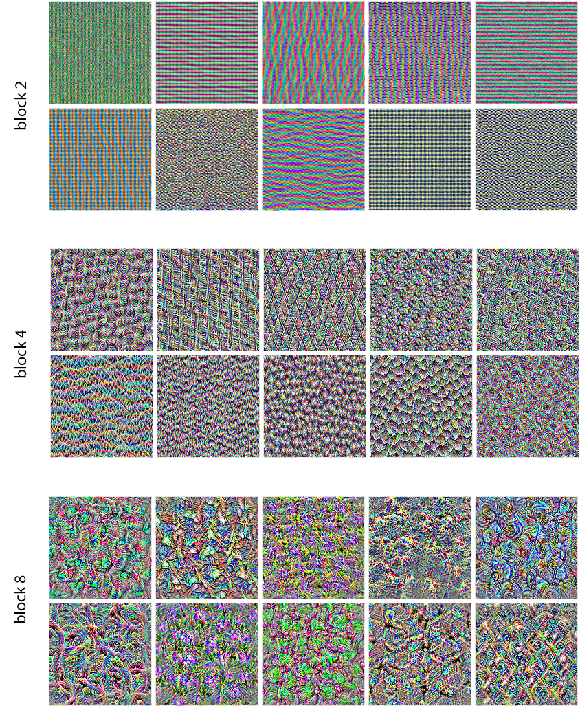
block2_sepconv1, block4_sepconv1, and block8_sepconv1
These filter visualizations tell you a lot about how ConvNet layers see the world: each layer in a ConvNet learns a collection of filters such that their inputs can be expressed as a combination of the filters. This is similar to how the Fourier transform decomposes signals onto a bank of cosine functions. The filters in these ConvNet filter banks get increasingly complex and refined as you go higher in the model:
- The filters from the first layers in the model encode simple directional edges and colors (or colored edges, in some cases).
- The filters from layers a bit further up the stack, such as
block4_sepconv1, encode simple textures made from combinations of edges and colors. - The filters in higher layers begin to resemble textures found in natural images: feathers, eyes, leaves, and so on.
Visualizing heatmaps of class activation
Here’s one last visualization technique — one that is useful for understanding which parts of a given image led a ConvNet to its final classification decision. This is helpful for “debugging” the decision process of a ConvNet, particularly in the case of a classification mistake (a problem domain called model interpretability). It can also allow you to locate specific objects in an image.
This general category of techniques is called class activation map (CAM) visualization, and it consists of producing heatmaps of class activation over input images. A class activation heatmap is a 2D grid of scores associated with a specific output class, computed for every location in any input image, indicating how important each location is with respect to the class under consideration. For instance, given an image fed into a dogs-versus-cats ConvNet, CAM visualization would allow you to generate a heatmap for the class “cat,” indicating how cat-like different parts of the image are, and also a heatmap for the class “dog,” indicating how dog-like parts of the image are. The specific implementation we’ll use is the one described in Selvaraju et al.[1]
Grad-CAM consists of taking the output feature map of a convolution layer, given an input image, and weighting every channel in that feature map by the gradient of the class with respect to the channel. Intuitively, one way to understand this trick is that you’re weighting a spatial map of “how intensely the input image activates different channels” by “how important each channel is with regard to the class,” resulting in a spatial map of “how intensely the input image activates the class.”
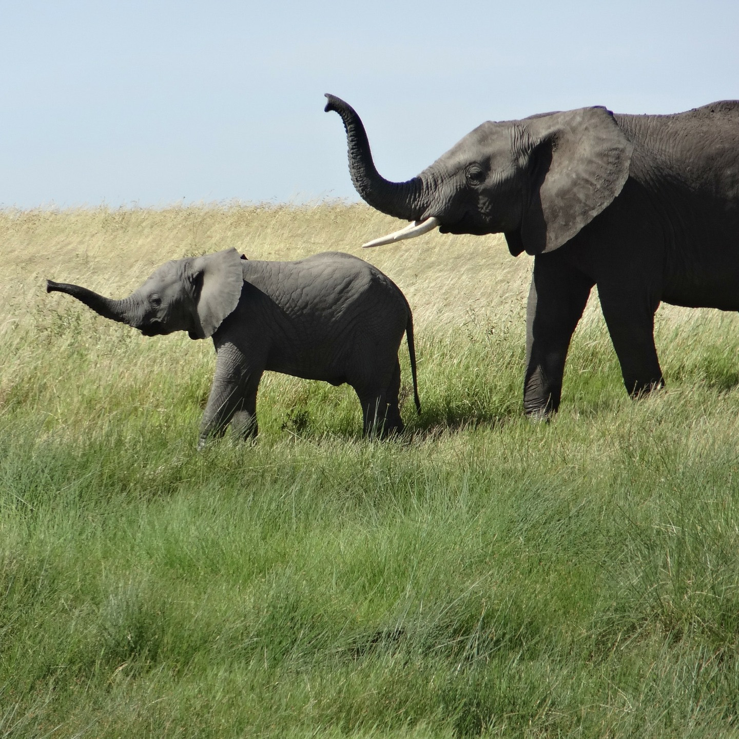
Let’s demonstrate this technique using the pretrained Xception model. Consider the image of two African elephants shown in figure 10.7, possibly a mother and her calf, strolling in the savanna. We can start by downloading this image and converting it to a NumPy array, as shown in figure 10.7.
# Downloads the image and stores it locally under the path img_path
img_path = keras.utils.get_file(
    fname="elephant.jpg",
    origin="https://img-datasets.s3.amazonaws.com/elephant.jpg",
)
# Returns a Python Imaging Library (PIL) image
img = keras.utils.load_img(img_path)
img_array = np.expand_dims(img, axis=0)
So far, we have only used KerasHub to instantiate a pretrained feature extractor network using the backbone class. For Grad-CAM, we need the entire Xception model including the classification head — recall that Xception was trained on the ImageNet dataset with ~1 million labeled images belonging to 1,000 different classes.
KerasHub provides a high-level task API for common end-to-end workflows like image classification, text classification, image generation, and so on. A task wraps preprocessing, a feature extraction network, and a task-specific head into a single class that is easy to use. Let’s try it out:
>>> model = keras_hub.models.ImageClassifier.from_preset( ... "xception_41_imagenet", ... # We can configure the final activation of the classifier. Here, ... # we use a softmax activation so our outputs are probabilities. ... activation="softmax", ... ) >>> preds = model.predict(img_array) >>> # ImageNet has 1,000 classes, so each prediction from our >>> # classifier has 1,000 entries. >>> preds.shape(1, 1000)>>> keras_hub.utils.decode_imagenet_predictions(preds)[[("African_elephant", 0.90331), ("tusker", 0.05487), ("Indian_elephant", 0.01637), ("triceratops", 0.00029), ("Mexican_hairless", 0.00018)]]
The top five classes predicted for this image are as follows:
- African elephant (with 90% probability)
- Tusker (with 5% probability)
- Indian elephant (with 2% probability)
- Triceratops and Mexican hairless dog with less than 0.1% probability
The network has recognized the image as containing an undetermined quantity of African elephants. The entry in the prediction vector that was maximally activated is the one corresponding to the “African elephant” class, at index 386:
>>> np.argmax(preds[0])386
To visualize which parts of the image are the most African elephant–like, let’s set up the Grad-CAM process.
You will note that we didn’t need to preprocess our image before calling the
task model. That’s because the KerasHub ImageClassifier is preprocessing inputs
for us as part of predict(). Let’s preprocess the image ourselves so
we can use the preprocessed inputs directly:
# KerasHub tasks like ImageClassifier have a preprocessor layer.
img_array = model.preprocessor(img_array)
First, we create a model that maps the input image to the activations of the last convolutional layer.
last_conv_layer_name = "block14_sepconv2_act"
last_conv_layer = model.backbone.get_layer(last_conv_layer_name)
last_conv_layer_model = keras.Model(model.inputs, last_conv_layer.output)
Second, we create a model that maps the activations of the last convolutional layer to the final class predictions.
classifier_input = last_conv_layer.output
x = classifier_input
for layer_name in ["pooler", "predictions"]:
    x = model.get_layer(layer_name)(x)
classifier_model = keras.Model(classifier_input, x)
Then, we compute the gradient of the top predicted class for our input image with respect to the activations of the last convolution layer. Once again, having to compute gradients means we have to use backend APIs.
Getting the gradient of the top class: TensorFlow version
Let’s start with the TensorFlow version, once again using GradientTape.
import tensorflow as tf

def get_top_class_gradients(img_array):
    # Computes activations of the last conv layer and makes the tape
    # watch it
    last_conv_layer_output = last_conv_layer_model(img_array)
    with tf.GradientTape() as tape:
        tape.watch(last_conv_layer_output)
        preds = classifier_model(last_conv_layer_output)
        top_pred_index = ops.argmax(preds[0])
        # Retrieves the activation channel corresponding to the top
        # predicted class
        top_class_channel = preds[:, top_pred_index]

    # Gets the gradient of the top predicted class with regard to the
    # output feature map of the last convolutional layer
    grads = tape.gradient(top_class_channel, last_conv_layer_output)
    return grads, last_conv_layer_output

grads, last_conv_layer_output = get_top_class_gradients(img_array)
grads = ops.convert_to_numpy(grads)
last_conv_layer_output = ops.convert_to_numpy(last_conv_layer_output)
Getting the gradient of the top class: PyTorch version
Next, here’s the PyTorch version, using .backward() and .grad.
def get_top_class_gradients(img_array):
    # Computes activations of the last conv layer
    last_conv_layer_output = last_conv_layer_model(img_array)
    # Creates a copy of last_conv_layer_output that we can get
    # gradients for
    last_conv_layer_output = (
        last_conv_layer_output.clone().detach().requires_grad_(True)
    )
    # Retrieves the activation channel corresponding to the top
    # predicted class
    preds = classifier_model(last_conv_layer_output)
    top_pred_index = ops.argmax(preds[0])
    top_class_channel = preds[:, top_pred_index]
    # Gets the gradient of the top predicted class with regard to the
    # output feature map of the last convolutional layer
    top_class_channel.backward()
    grads = last_conv_layer_output.grad
    return grads, last_conv_layer_output

grads, last_conv_layer_output = get_top_class_gradients(img_array)
grads = ops.convert_to_numpy(grads)
last_conv_layer_output = ops.convert_to_numpy(last_conv_layer_output)
Getting the gradient of the top class: JAX version
Finally, let’s do JAX. We define a separate loss computation function that takes the final layer’s output and returns the activation channel corresponding to the top predicted class. We use this activation value as our loss, allowing us to compute the gradient.
import jax

# Defines a separate loss function
def loss_fn(last_conv_layer_output):
    preds = classifier_model(last_conv_layer_output)
    top_pred_index = ops.argmax(preds[0])
    top_class_channel = preds[:, top_pred_index]
    # Returns the activation value of the top-class channel
    return top_class_channel[0]

# Creates a gradient function
grad_fn = jax.grad(loss_fn)

def get_top_class_gradients(img_array):
    last_conv_layer_output = last_conv_layer_model(img_array)
    # Now  retrieving the gradient of the top-class channel is just a
    # matter of calling the gradient function!
    grads = grad_fn(last_conv_layer_output)
    return grads, last_conv_layer_output

grads, last_conv_layer_output = get_top_class_gradients(img_array)
grads = ops.convert_to_numpy(grads)
last_conv_layer_output = ops.convert_to_numpy(last_conv_layer_output)
Displaying the class activation heatmap
Now, we apply pooling and importance weighting to the gradient tensor to obtain our heatmap of class activation.
# This is a vector where each entry is the mean intensity of the
# gradient for a given channel. It quantifies the importance of each
# channel with regard to the top predicted class.
pooled_grads = np.mean(grads, axis=(0, 1, 2))
last_conv_layer_output = last_conv_layer_output[0].copy()
# Multiplies each channel in the output of the last convolutional layer
# by how important this channel is
for i in range(pooled_grads.shape[-1]):
    last_conv_layer_output[:, :, i] *= pooled_grads[i]
# The channel-wise mean of the resulting feature map is our heatmap of
# class activation.
heatmap = np.mean(last_conv_layer_output, axis=-1)
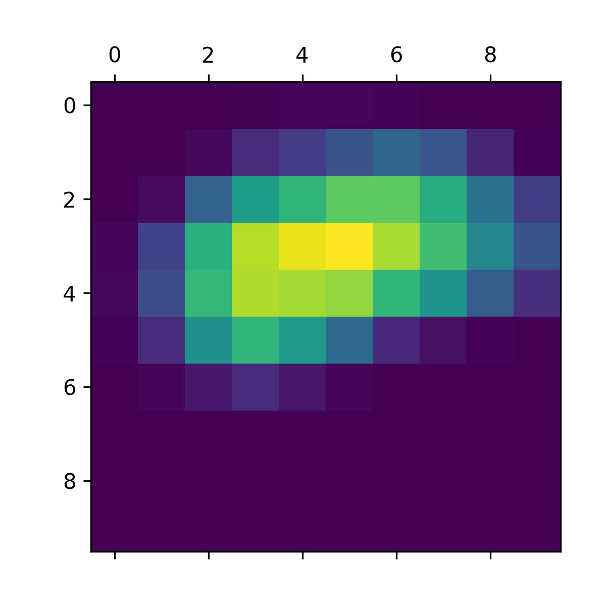
For visualization purposes, you’ll also normalize the heatmap between 0 and 1. The result is shown in figure 10.8.
heatmap = np.maximum(heatmap, 0)
heatmap /= np.max(heatmap)
plt.matshow(heatmap)
Finally, let’s generate an image that superimposes the original image on the heatmap you just obtained (see figure 10.9).
import matplotlib.cm as cm

# Loads the original image
img = keras.utils.load_img(img_path)
img = keras.utils.img_to_array(img)

# Rescales the heatmap to the range 0–255
heatmap = np.uint8(255 * heatmap)

# Uses the "jet" colormap to recolorize the heatmap
jet = cm.get_cmap("jet")
jet_colors = jet(np.arange(256))[:, :3]
jet_heatmap = jet_colors[heatmap]

# Creates an image that contains the recolorized heatmap
jet_heatmap = keras.utils.array_to_img(jet_heatmap)
jet_heatmap = jet_heatmap.resize((img.shape[1], img.shape[0]))
jet_heatmap = keras.utils.img_to_array(jet_heatmap)

# Superimposes the heatmap and the original image, with the heatmap at
# 40% opacity
superimposed_img = jet_heatmap * 0.4 + img
superimposed_img = keras.utils.array_to_img(superimposed_img)

# Shows the superimposed image
plt.imshow(superimposed_img)
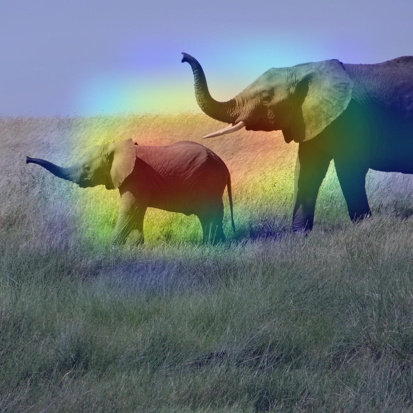
This visualization technique answers two important questions:
- Why did the network think this image contained an African elephant?
- Where is the African elephant located in the picture?
In particular, it’s interesting to note that the ears of the elephant calf are strongly activated: this is probably how the network can tell the difference between African and Indian elephants.
Summary
- ConvNets process images by applying a set of learned filters. Filters from earlier layers detect edges and basic textures, while filters from later layers detect increasingly abstract concepts.
- You can visualize both the pattern that a filter detects and a filter’s response map across an image.
- You can use the Grad-CAM technique to visualize what area(s) in an image were responsible for a classifier’s decision.
- Together, these techniques make ConvNets highly interpretable.