


Chapter 8 gave you a first introduction to deep learning for computer vision via a simple use case: binary image classification. But there’s more to computer vision than image classification! This chapter dives deeper into another essential computer vision application — image segmentation.
Computer vision tasks
So far, we’ve focused on image classification models: an image goes in, a label comes out. “This image likely contains a cat; this other one likely contains a dog.” But image classification is only one of several possible applications of deep learning in computer vision. In general, there are three essential computer vision tasks you need to know about:
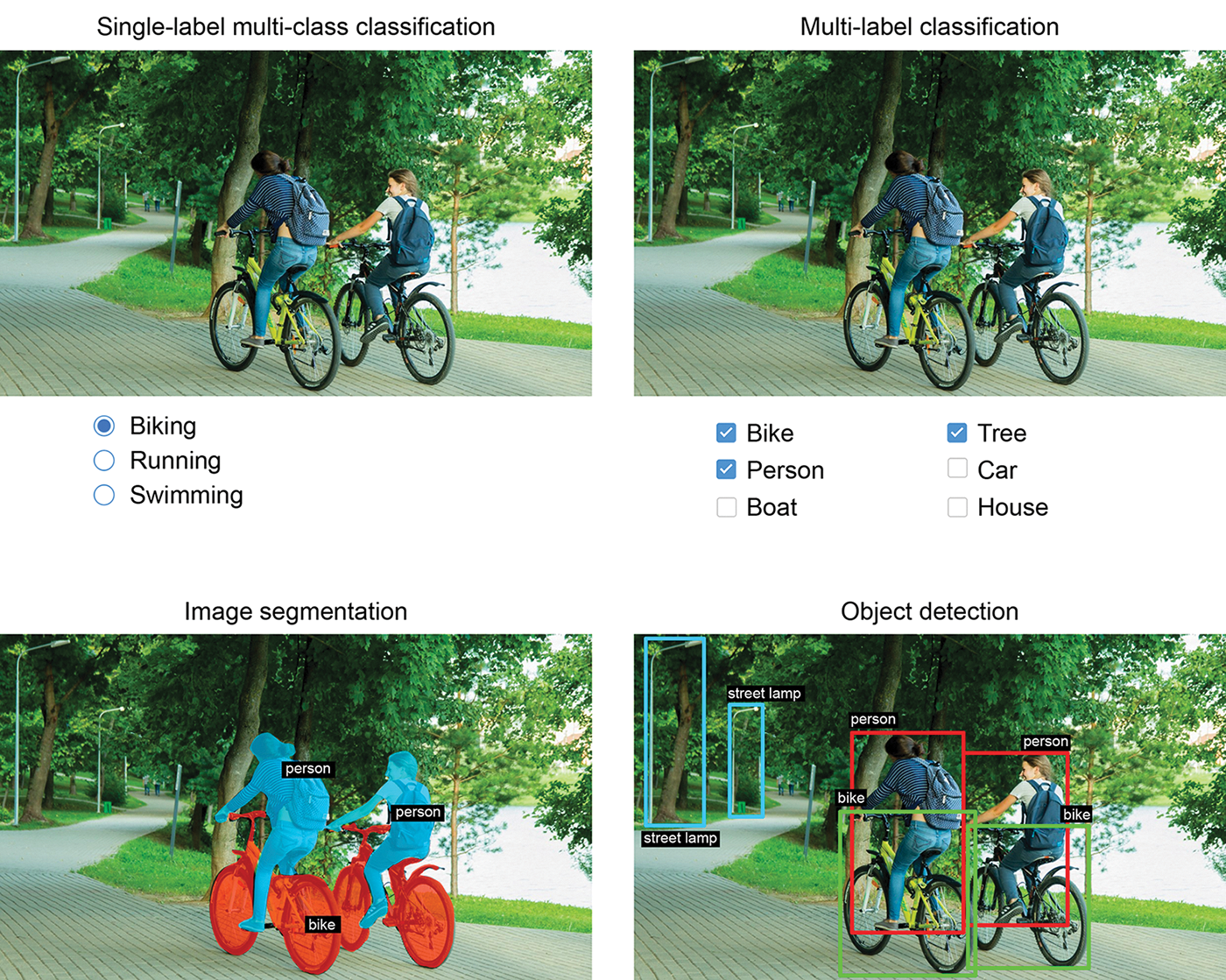
- Image classification, where the goal is to assign one or more labels to an image. It may be either single-label classification (meaning categories are mutually exclusive) or multilabel classification (tagging all categories that an image belongs to, as shown in figure 11.1). For example, when you search for a keyword on the Google Photos app, behind the scenes you’re querying a very large multilabel classification model — one with over 20,000 different classes, trained on millions of images.
- Image segmentation, where the goal is to “segment” or “partition” an image into different areas, with each area usually representing a category (as shown in figure 11.1). For instance, when Zoom or Google Meet displays a custom background behind you in a video call, it’s using an image segmentation model to distinguish your face from what’s behind it, with pixel-level precision.
- Object detection, where the goal is to draw rectangles (called bounding boxes) around objects of interest in an image and associate each rectangle with a class. A self-driving car could use an object detection model to monitor cars, pedestrians, and signs in view of its cameras, for instance.
Deep learning for computer vision also encompasses a number of somewhat more niche tasks besides these three, such as image similarity scoring (estimating how visually similar two images are), keypoint detection (pinpointing attributes of interest in an image, such as facial features), pose estimation, 3D mesh estimation, depth estimation, and so on. But to start with, image classification, image segmentation, and object detection form the foundation that every machine learning engineer should be familiar with. Almost all computer vision applications boil down to one of these three.
You’ve seen image classification in action in Chapter 8. Next, let’s dive into image segmentation. It’s a very useful and very versatile technique, and you can straightforwardly approach it with what you’ve already learned so far. Then, in the next chapter, you’ll learn about object detection in detail.
Types of image segmentation
Image segmentation with deep learning is about using a model to assign a class to each pixel in an image, thus segmenting the image into different zones (such as “background” and “foreground” or “road,” “car,” and “sidewalk”). This general category of techniques can be used to power a considerable variety of valuable applications in image and video editing, autonomous driving, robotics, medical imaging, and so on.
There are three different flavors of image segmentation that you should know about:
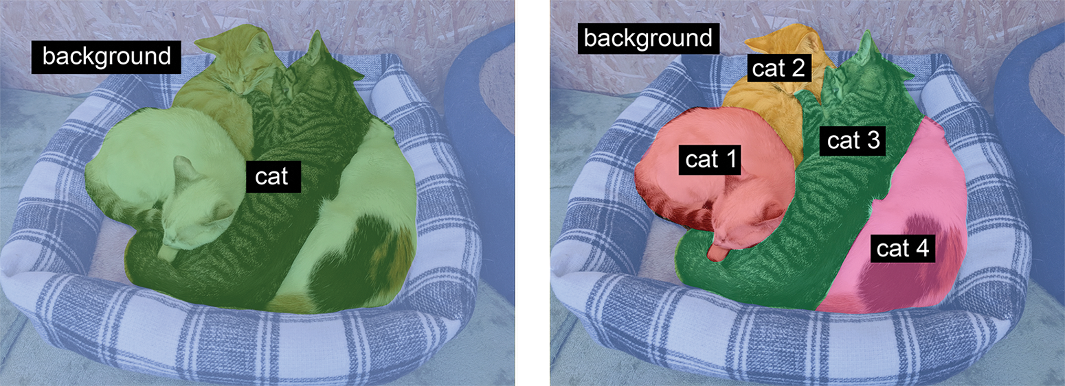
- Semantic segmentation, where each pixel is independently classified into a semantic category, like “cat.” If there are two cats in the image, the corresponding pixels are all mapped to the same generic “cat” category (see figure 11.2).
- Instance segmentation, which seeks to parse out individual object instances. In an image with two cats in it, instance segmentation would distinguish between pixels belonging to “cat 1” and pixels belonging to “cat 2” (see figure 11.2).
- Panoptic segmentation, which combines semantic segmentation and instance segmentation by assigning to each pixel in an image both a semantic label (like “cat”) and an instance label (like “cat 2”). This is the most informative of all three segmentation types.
To get more familiar with segmentation, let’s get started with training a small segmentation model from scratch on your own data.
Training a segmentation model from scratch
In this first example, we’ll focus on semantic segmentation. We’ll be looking once again at images of cats and dogs, and this time we’ll be learning to tell apart the main subject and its background.
Downloading a segmentation dataset
We’ll work with the Oxford-IIIT Pets dataset (https://www.robots.ox.ac.uk/~vgg/data/pets/), which contains 7,390 pictures of various breeds of cats and dogs, together with foreground-background segmentation masks for each picture. A segmentation mask is the image segmentation equivalent of a label: it’s an image the same size as the input image, with a single color channel where each integer value corresponds to the class of the corresponding pixel in the input image. In our case, the pixels of our segmentation masks can take one of three integer values:
- 1 (foreground)
- 2 (background)
- 3 (contour)
Let’s start by downloading and uncompressing our dataset, using the wget and tar
shell utilities:
!wget http://www.robots.ox.ac.uk/~vgg/data/pets/data/images.tar.gz
!wget http://www.robots.ox.ac.uk/~vgg/data/pets/data/annotations.tar.gz
!tar -xf images.tar.gz
!tar -xf annotations.tar.gz
The input pictures are stored as JPG files in the images/ folder
(such as images/Abyssinian_1.jpg), and the corresponding segmentation mask
is stored as a PNG file with the same name in the annotations/trimaps/ folder
(such as annotations/trimaps/Abyssinian_1.png).
Let’s prepare the list of input file paths, as well as the list of the corresponding mask file paths:
import pathlib

input_dir = pathlib.Path("images")
target_dir = pathlib.Path("annotations/trimaps")

input_img_paths = sorted(input_dir.glob("*.jpg"))
# Ignores some spurious files in the trimaps directory that start with
# a "."
target_paths = sorted(target_dir.glob("[!.]*.png"))
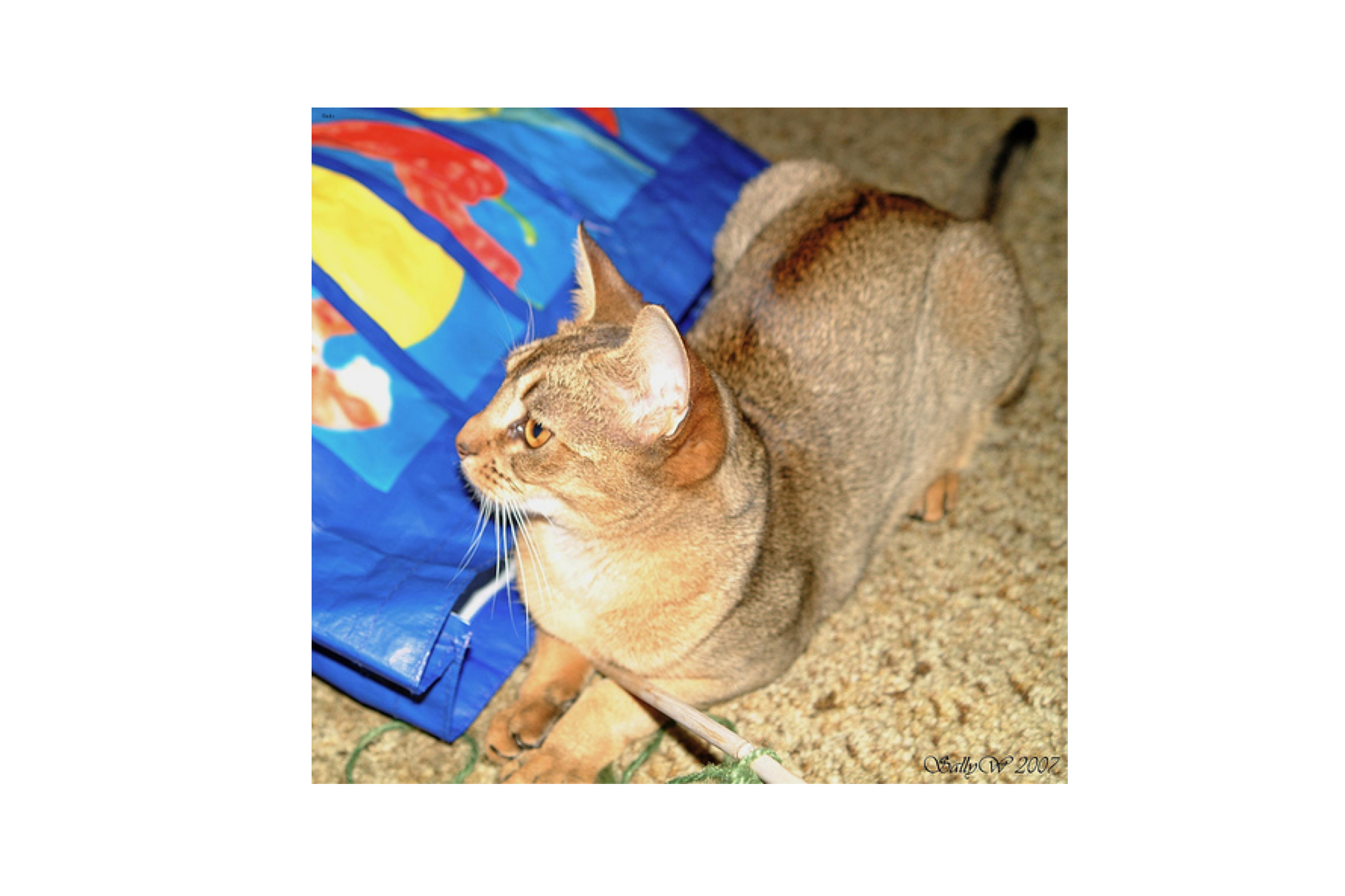
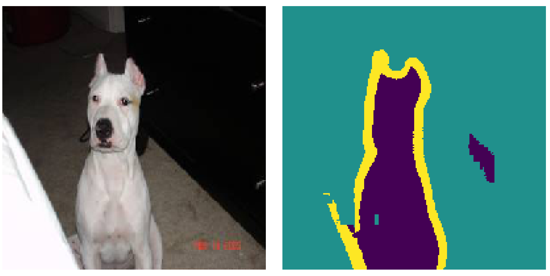
Now, what does one of these inputs and its mask look like? Let’s take a quick look (see figure 11.3).
import matplotlib.pyplot as plt
from keras.utils import load_img, img_to_array, array_to_img

plt.axis("off")
# Displays input image number 9
plt.imshow(load_img(input_img_paths[9]))
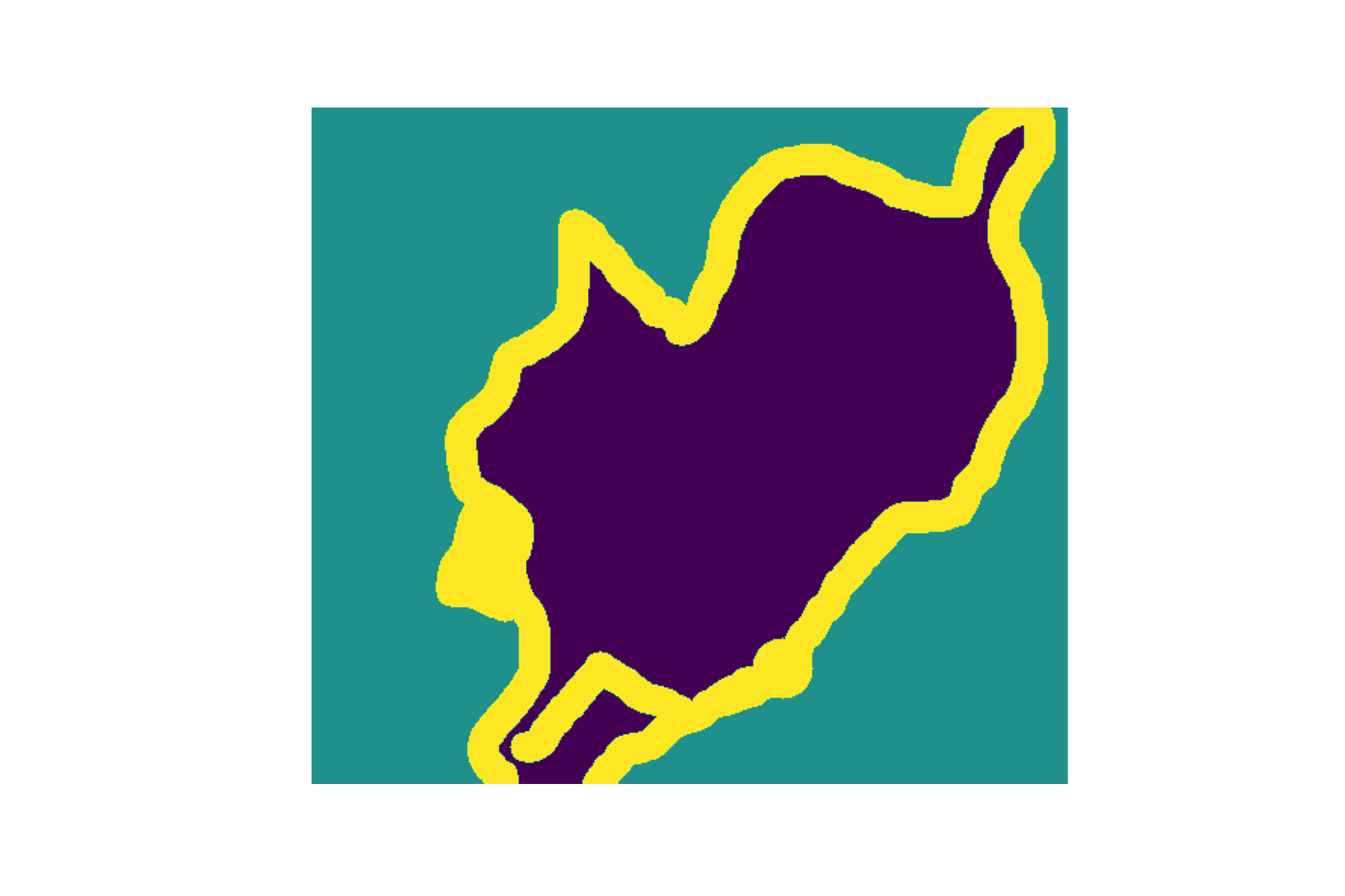
Let’s look at its target mask as well (see figure 11.4):
def display_target(target_array):
    # The original labels are 1, 2, and 3. We subtract 1 so that the
    # labels range from 0 to 2, and then we multiply by 127 so that the
    # labels become 0 (black), 127 (gray), 254 (near-white).
    normalized_array = (target_array.astype("uint8") - 1) * 127
    plt.axis("off")
    plt.imshow(normalized_array[:, :, 0])

# We use color_mode='grayscale' so that the image we load is treated as
# having a single color channel.
img = img_to_array(load_img(target_paths[9], color_mode="grayscale"))
display_target(img)
Next, let’s load our inputs and targets into two NumPy arrays. Since the dataset is very small, we can load everything into memory:
import numpy as np
import random

# We resize everything to 200 x 200 for this example.
img_size = (200, 200)
# Total number of samples in the data
num_imgs = len(input_img_paths)

# Shuffles the file paths (they were originally sorted by breed). We
# use the same seed (1337) in both statements to ensure that the input
# paths and target paths stay in the same order.
random.Random(1337).shuffle(input_img_paths)
random.Random(1337).shuffle(target_paths)

def path_to_input_image(path):
    return img_to_array(load_img(path, target_size=img_size))

def path_to_target(path):
    img = img_to_array(
        load_img(path, target_size=img_size, color_mode="grayscale")
    )
    # Subtracts 1 so that our labels become 0, 1, and 2
    img = img.astype("uint8") - 1
    return img

# Loads all images in the input_imgs float32 array and their masks in
# the targets uint8 array (same order). The inputs have three channels
# (RGB values), and the targets have a single channel (which contains
# integer labels).
input_imgs = np.zeros((num_imgs,) + img_size + (3,), dtype="float32")
targets = np.zeros((num_imgs,) + img_size + (1,), dtype="uint8")
for i in range(num_imgs):
    input_imgs[i] = path_to_input_image(input_img_paths[i])
    targets[i] = path_to_target(target_paths[i])
As always, let’s split the arrays into a training and a validation set:
# Reserves 1,000 samples for validation
num_val_samples = 1000
# Splits the data into a training and a validation set
train_input_imgs = input_imgs[:-num_val_samples]
train_targets = targets[:-num_val_samples]
val_input_imgs = input_imgs[-num_val_samples:]
val_targets = targets[-num_val_samples:]
Building and training the segmentation model
Now, it’s time to define our model:
import keras
from keras.layers import Rescaling, Conv2D, Conv2DTranspose

def get_model(img_size, num_classes):
    inputs = keras.Input(shape=img_size + (3,))
    # Don't forget to rescale input images to the [0–1] range.
    x = Rescaling(1.0 / 255)(inputs)

    # We use padding="same" everywhere to avoid the influence of border
    # padding on feature map size.
    x = Conv2D(64, 3, strides=2, activation="relu", padding="same")(x)
    x = Conv2D(64, 3, activation="relu", padding="same")(x)
    x = Conv2D(128, 3, strides=2, activation="relu", padding="same")(x)
    x = Conv2D(128, 3, activation="relu", padding="same")(x)
    x = Conv2D(256, 3, strides=2, padding="same", activation="relu")(x)
    x = Conv2D(256, 3, activation="relu", padding="same")(x)

    x = Conv2DTranspose(256, 3, activation="relu", padding="same")(x)
    x = Conv2DTranspose(256, 3, strides=2, activation="relu", padding="same")(x)
    x = Conv2DTranspose(128, 3, activation="relu", padding="same")(x)
    x = Conv2DTranspose(128, 3, strides=2, activation="relu", padding="same")(x)
    x = Conv2DTranspose(64, 3, activation="relu", padding="same")(x)
    x = Conv2DTranspose(64, 3, strides=2, activation="relu", padding="same")(x)

    # We end the model with a per-pixel three-way softmax to classify
    # each output pixel into one of our three categories.
    outputs = Conv2D(num_classes, 3, activation="softmax", padding="same")(x)

    return keras.Model(inputs, outputs)

model = get_model(img_size=img_size, num_classes=3)
The first half of the model closely resembles the kind of ConvNet you’d use for image
classification: a stack of Conv2D layers, with gradually increasing filter sizes.
We downsample our images three times by a factor of
two each — ending up with activations of size
(25, 25, 256). The purpose of this first half is to encode the images into
smaller feature maps, where each spatial location (or “pixel”) contains
information about a large spatial chunk of the original image. You can understand
it as a kind of compression.
One important difference between the first half of this model and the classification models
you’ve seen before is the way we do downsampling: in the classification ConvNets
from chapter 8, we used MaxPooling2D layers to downsample feature maps.
Here, we downsample by adding strides to every other convolution layer (if you
don’t remember the details of how convolution strides work, see
chapter 8, section 8.1.1). We do this because,
in the case of image segmentation, we care a lot about the spatial location of
information in the image since we need to produce per-pixel target masks as
output of the model. When you do 2 × 2 max pooling, you are completely destroying
location information within each pooling window: you return one scalar value
per window, with zero knowledge of which of the four locations in the windows
the value came from.
So, while max pooling layers perform well for classification tasks, they would hurt us quite a bit for a segmentation task. Meanwhile, strided convolutions do a better job at downsampling feature maps while retaining location information. Throughout this book, you’ll notice that we tend to use strides instead of max pooling in any model that cares about feature location, such as the generative models in chapter 17.
The second half of the model is a stack of Conv2DTranspose layers. What are those?
Well, the output of the first half of the model is a feature map of shape (25, 25, 256),
but we want our final output to predict a class for each pixel, matching the original
spatial dimensions. The final model output will have shape (200, 200, num_classes),
which is (200, 200, 3) here. Therefore, we need to apply a kind of inverse of the
transformations we’ve applied so far, something that will upsample the feature
maps instead of downsampling them. That’s the purpose of the Conv2DTranspose layer:
you can think of it as a kind of convolution layer that learns to upsample.
If you have an input of shape (100, 100, 64) and you run it
through the layer Conv2D(128, 3, strides=2, padding="same"), you get an
output of shape (50, 50, 128). If you run this output through the layer
Conv2DTranspose(64, 3, strides=2, padding="same"), you get back an output
of shape (100, 100, 64), the same as the original. So after compressing
our inputs into feature maps of shape (25, 25, 256) via a stack of Conv2D
layers, we can simply apply the corresponding sequence of Conv2DTranspose
layers followed by a final Conv2D layer to produce outputs of shape (200, 200, 3).
To evaluate the model, we’ll use a metric named Intersection over Union (IoU). It’s a measure of the match between the ground truth segmentation masks and the predicted masks. It can be computed separately for each class or averaged over multiple classes. Here’s how it works:
- Compute the intersection between the masks, the area where the prediction and ground truth overlap.
- Compute the union of the masks, the total area covered by both masks combined. This is the whole space we’re interested in — the target object and any extra bits your model might have included by mistake.
- Divide the intersection area by the union area to get the IoU. It’s a number between 0 and 1, where 1 denotes a perfect match, and 0 denotes a complete miss.
We can simply use a built-in Keras metric rather than building this ourselves:
foreground_iou = keras.metrics.IoU(
    # Specifies the total number of classes
    num_classes=3,
    # Specifies the class to compute IoU for (0 = foreground)
    target_class_ids=(0,),
    name="foreground_iou",
    # Our targets are sparse (integer class IDs).
    sparse_y_true=True,
    # But our model's predictions are a dense softmax!
    sparse_y_pred=False,
)
We can now compile and fit our model:
model.compile(
    optimizer="adam",
    loss="sparse_categorical_crossentropy",
    metrics=[foreground_iou],
)
callbacks = [
    keras.callbacks.ModelCheckpoint(
        "oxford_segmentation.keras",
        save_best_only=True,
    ),
]
history = model.fit(
    train_input_imgs,
    train_targets,
    epochs=50,
    callbacks=callbacks,
    batch_size=64,
    validation_data=(val_input_imgs, val_targets),
)
Let’s display our training and validation loss (see figure 11.5):
epochs = range(1, len(history.history["loss"]) + 1)
loss = history.history["loss"]
val_loss = history.history["val_loss"]
plt.figure()
plt.plot(epochs, loss, "r--", label="Training loss")
plt.plot(epochs, val_loss, "b", label="Validation loss")
plt.title("Training and validation loss")
plt.legend()
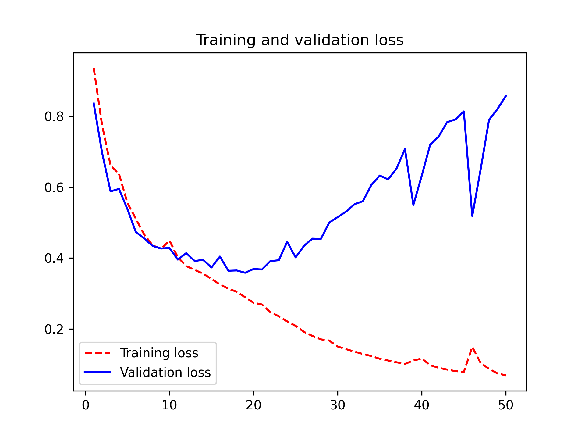
You can see that we start overfitting midway, around epoch 25. Let’s reload our best-performing model according to validation loss and demonstrate how to use it to predict a segmentation mask (see figure 11.6):
model = keras.models.load_model("oxford_segmentation.keras")

i = 4
test_image = val_input_imgs[i]
plt.axis("off")
plt.imshow(array_to_img(test_image))

mask = model.predict(np.expand_dims(test_image, 0))[0]

# Utility to display a model's prediction
def display_mask(pred):
    mask = np.argmax(pred, axis=-1)
    mask *= 127
    plt.axis("off")
    plt.imshow(mask)

display_mask(mask)
There are a couple of small artifacts in our predicted mask, caused by geometric shapes in the foreground and background. Nevertheless, our model appears to work nicely.
Using a pretrained segmentation model
In the image classification example from chapter 8, you saw how using a pretrained model could significantly boost your accuracy — especially when you only have a few samples to train on. Image segmentation is no different.
The Segment Anything Model,[1] or SAM for short, is a powerful pretrained segmentation model you can use for, well, almost anything. It was developed by Meta AI and released in April 2023. It was trained on 11 million images and their segmentation masks, covering over 1 billion object instances. This massive amount of training data provides the model with built-in knowledge of virtually any object that appears in natural images.
The main innovation of SAM is that it’s not limited to a predefined set of object classes. You can use it for segmenting new objects simply by providing an example of what you’re looking for. You don’t even need to fine-tune the model first. Let’s see how that works.
Downloading the Segment Anything Model
First, let’s instantiate SAM and download its weights. Once again, we can use the KerasHub package to use this pretrained model without needing to implement it ourselves from scratch.
Remember the ImageClassifier task we used in the previous chapter? We can use another
KerasHub task ImageSegmenter for wrapping pretrained image segmentation models
into a high-level model with standard inputs and outputs. Here, we’ll use the
sam_huge_sa1b pretrained model, where sam stands for the model, huge
refers to the number of parameters in the model, and sa1b stands for the SA-1B
dataset released along with the model, with 1 billion annotated masks. Let’s
download it now:
import keras_hub

model = keras_hub.models.ImageSegmenter.from_preset("sam_huge_sa1b")
One thing we can note off the bat is that our model is, indeed, huge:
>>> model.count_params()641090864
At 641 million parameters, SAM is the largest model we have used so far in this book. The trend of pretrained models getting larger and larger and using more and more data will be discussed in more detail in chapter 16.
How Segment Anything works
Before we try running some segmentation with the model, let’s talk a little more about how SAM works. Much of the capability of the model comes from the scale of the pretraining dataset. Meta developed the SA-1B dataset along with the model, where the partially trained model was used to assist with the data labeling process. That is, the dataset and model were developed together in a feedback loop of sorts.
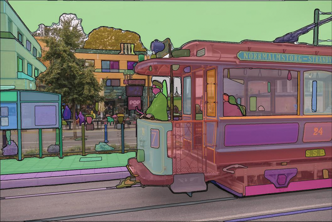
The goal with the SA-1B dataset is to create fully segmented images, where every object in an image is given a unique segmentation mask. See figure 11.7 as an example. Each image in the dataset has ~100 masks on average, and some images have over 500 individually masked objects. This was done through a pipeline of increasingly automated data collection. At first, human experts manually segmented a small example dataset of images, which was used to train an initial model. This model was used to help drive a semiautomated stage of data collection, where images were first segmented by SAM and improved by human correction and further annotation.
The model is trained on (image, prompt, mask) triples. image and prompt
are the model inputs. The image can be any input image, and the prompt can take a
couple of forms:
- A point inside the object to mask
- A box around the object to mask
Given the image and prompt input, the model is expected to produce an
accurate predicted mask for the object indicated by the prompt, which is
compared with a ground truth mask label.
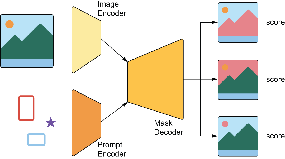
The model consists of a few separate components. An image encoder similar to the Xception model we used in previous chapters, will take an input image and output a much smaller image embedding. This is something we already know how to build.
Next, we add a prompt encoder, which is responsible for mapping prompts in any of the previously mentioned forms to an embedded vector, and a mask decoder, which takes in both the image embedding and prompt embedding and outputs a few possible predicted masks. We won’t get into the details of the prompt encoder and mask decoder here, as they use some modeling techniques we won’t see until later chapters. We can compare these predicted masks with our ground truth mask much like we did in the earlier section of this chapter (see figure 11.8).
All of these subcomponents are trained simultaneously by forming batches of new
(image, prompt, mask) triples to train on from the SA-1B image and mask data.
The process here is actually quite simple. For a given input image, choose a
random mask in the input. Next, randomly choose whether to create a box prompt
or a point prompt. To create a point prompt, choose a random pixel inside the
mask label. To create a box prompt, draw a box around all points inside
the mask label. We can repeat this process indefinitely, sampling a number of
(image, prompt, mask) triples from each image input.
Preparing a test image
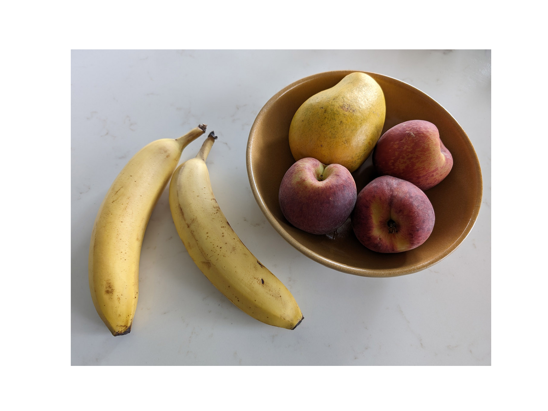
Let’s make this a little more concrete by trying the model out. We can start by loading a test image for our segmentation work. We’ll use a picture of a bowl of fruits (see figure 11.9):
# Downloads the image and returns the local file path
path = keras.utils.get_file(
    origin="https://s3.amazonaws.com/keras.io/img/book/fruits.jpg"
)
# Loads the image as a Python Imaging Library (PIL) object
pil_image = keras.utils.load_img(path)
# Turns the PIL object into a NumPy matrix
image_array = keras.utils.img_to_array(pil_image)

# Displays the NumPy matrix
plt.imshow(image_array.astype("uint8"))
plt.axis("off")
plt.show()
SAM expects inputs that are 1024 × 1024. However, forcibly resizing arbitrary images
to 1024 × 1024 would distort their aspect ratio — for instance, our image isn’t square.
It’s better to first resize the image so that its longest side becomes 1,024 pixels long and then pad
the remaining pixels with a filler value, such as 0. We can achieve this with the pad_to_aspect_ratio
argument in the keras.ops.image.resize() operation, like this:
from keras import ops

image_size = (1024, 1024)

def resize_and_pad(x):
    return ops.image.resize(x, image_size, pad_to_aspect_ratio=True)

image = resize_and_pad(image_array)
Next, let’s define a few utilities that will come in handy when using the model. We’re going to need to
- Display images.
- Display segmentation masks overlaid on an image.
- Highlight specific points on an image.
- Display boxes overlaid on an image.
All our utilities take a Matplotlib axis object (noted ax) so that they can all write to the same figure:
import matplotlib.pyplot as plt
from keras import ops

def show_image(image, ax):
    ax.imshow(ops.convert_to_numpy(image).astype("uint8"))

def show_mask(mask, ax):
    color = np.array([30 / 255, 144 / 255, 255 / 255, 0.6])
    h, w, _ = mask.shape
    mask_image = mask.reshape(h, w, 1) * color.reshape(1, 1, -1)
    ax.imshow(mask_image)

def show_points(points, ax):
    x, y = points[:, 0], points[:, 1]
    ax.scatter(x, y, c="green", marker="*", s=375, ec="white", lw=1.25)

def show_box(box, ax):
    box = box.reshape(-1)
    x0, y0 = box[0], box[1]
    w, h = box[2] - box[0], box[3] - box[1]
    ax.add_patch(plt.Rectangle((x0, y0), w, h, ec="red", fc="none", lw=2))
Prompting the model with a target point
To use SAM, you need to prompt it. This means we need one of the following:
- Point prompts — Select a point in an image and let the model segment the object that the point belongs to.
- Box prompts — Draw an approximate box around an object (it does not need to be particularly precise) and let the model segment the object in the box.
Let’s start with a point prompt. Points are labeled, with 1 indicating the foreground (the object you want to segment) and 0 indicating the background (everything around the object). In ambiguous cases, to improve your results, you could pass multiple labeled points, instead of a single point, to refine your definition of what should be included (points labeled 1) and what should be excluded (points labeled 0).
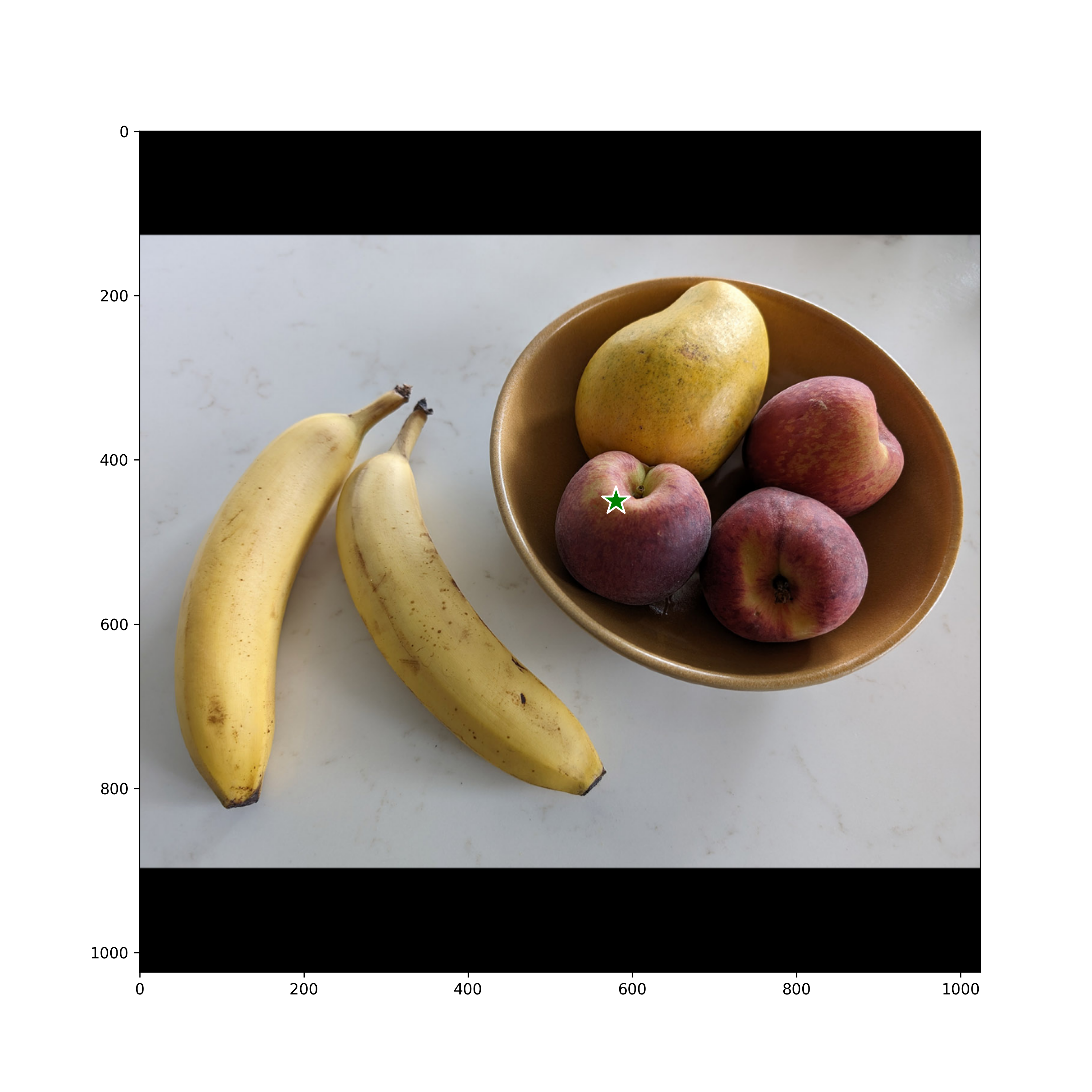
We try a single foreground point (see figure 11.10). Here’s a test point:
import numpy as np

# Coordinates of our point
input_point = np.array([[580, 450]])
# 1 means foreground, and 0 means background.
input_label = np.array([1])

plt.figure(figsize=(10, 10))
# "gca" means "get current axis" — the current figure.
show_image(image, plt.gca())
show_points(input_point, plt.gca())
plt.show()
Let’s prompt SAM with it:
outputs = model.predict(
    {
        "images": ops.expand_dims(image, axis=0),
        "points": ops.expand_dims(input_point, axis=0),
        "labels": ops.expand_dims(input_label, axis=0),
    }
)
The return value outputs has a "masks" field which contains four 256 × 256 candidate masks for the target object,
ranked by decreasing match quality. The quality scores of the masks are available under the "iou_pred" field as part of the model’s output:
>>> outputs["masks"].shape(1, 4, 256, 256)
Let’s overlay the first mask on the image (see figure 11.11):
def get_mask(sam_outputs, index=0):
    mask = sam_outputs["masks"][0][index]
    mask = np.expand_dims(mask, axis=-1)
    mask = resize_and_pad(mask)
    return ops.convert_to_numpy(mask) > 0.0

mask = get_mask(outputs, index=0)

plt.figure(figsize=(10, 10))
show_image(image, plt.gca())
show_mask(mask, plt.gca())
show_points(input_point, plt.gca())
plt.show()
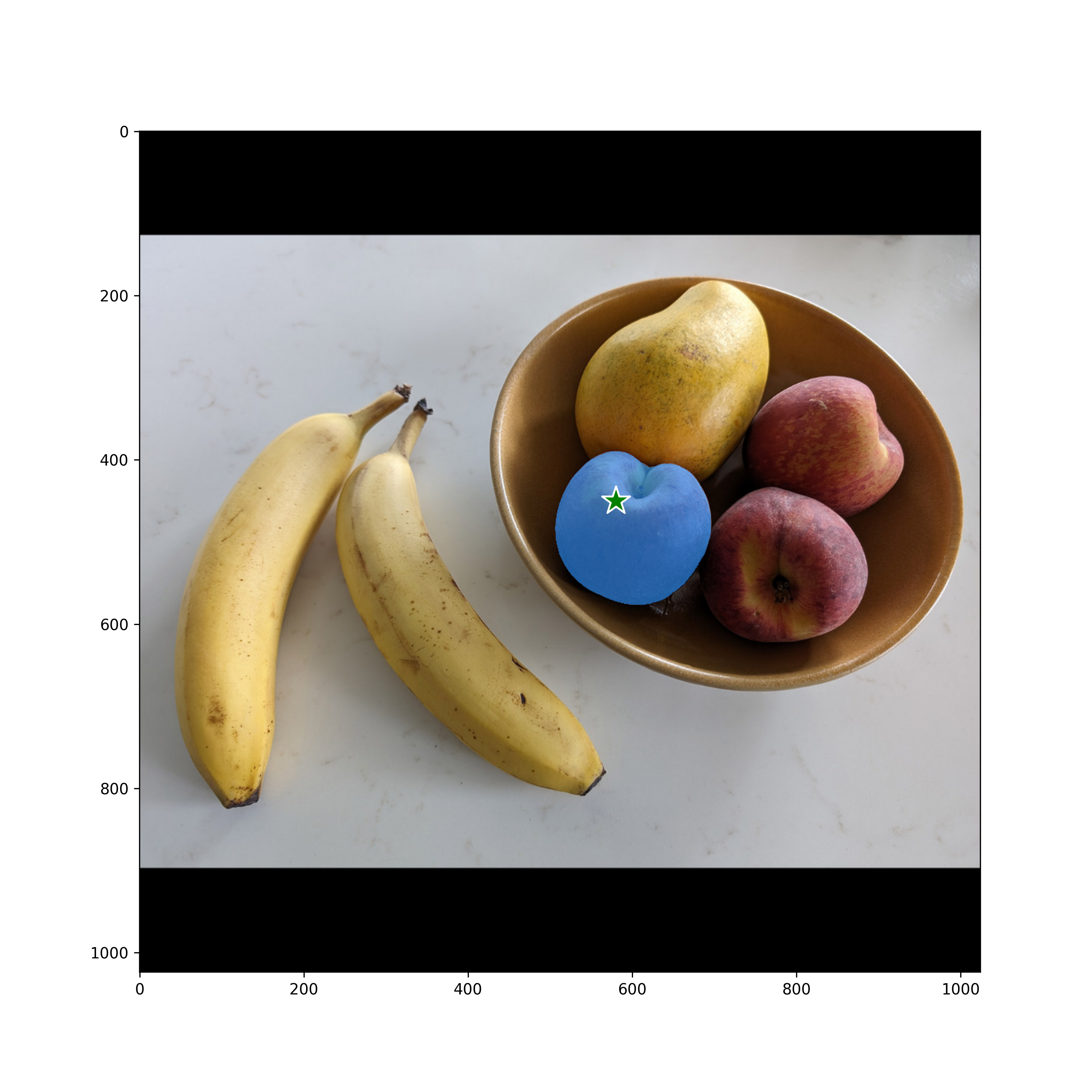
Pretty good!
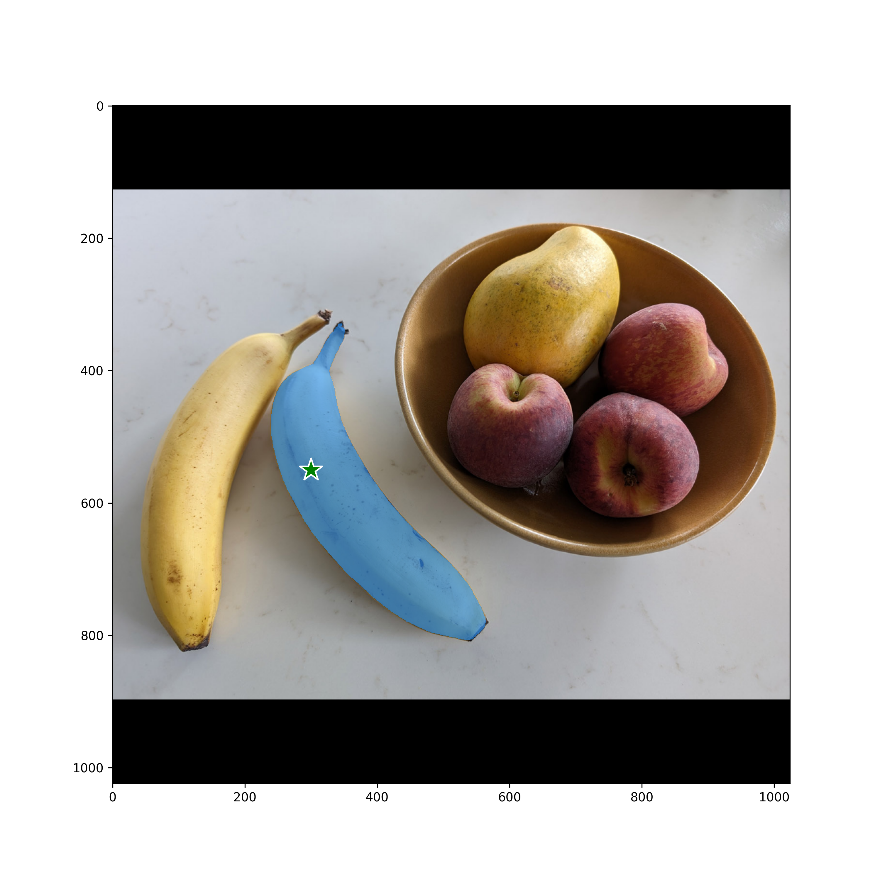
Next, let’s try a banana. We’ll prompt the model with coordinates (300, 550),
which land on the second banana from the left (see figure 11.12):
input_point = np.array([[300, 550]])
input_label = np.array([1])

outputs = model.predict(
    {
        "images": ops.expand_dims(image, axis=0),
        "points": ops.expand_dims(input_point, axis=0),
        "labels": ops.expand_dims(input_label, axis=0),
    }
)
mask = get_mask(outputs, index=0)

plt.figure(figsize=(10, 10))
show_image(image, plt.gca())
show_mask(mask, plt.gca())
show_points(input_point, plt.gca())
plt.show()
Now, what about the other mask candidates? Those can come in handy for ambiguous prompts. Let’s try to plot the other three masks (see figure 11.13):
fig, axes = plt.subplots(1, 3, figsize=(20, 60))
masks = outputs["masks"][0][1:]
for i, mask in enumerate(masks):
    show_image(image, axes[i])
    show_points(input_point, axes[i])
    mask = get_mask(outputs, index=i + 1)
    show_mask(mask, axes[i])
    axes[i].set_title(f"Mask {i + 1}", fontsize=16)
    axes[i].axis("off")
plt.show()
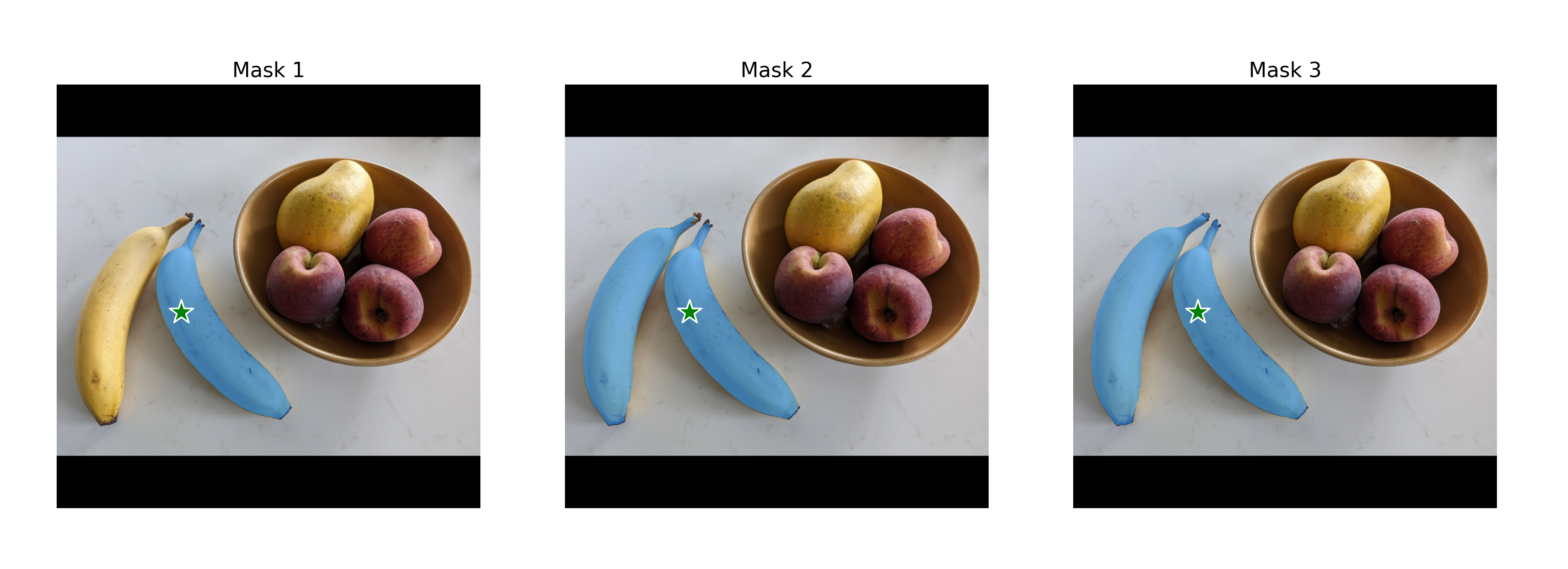
As you can see here, an alternative segmentation found by the model includes both bananas.
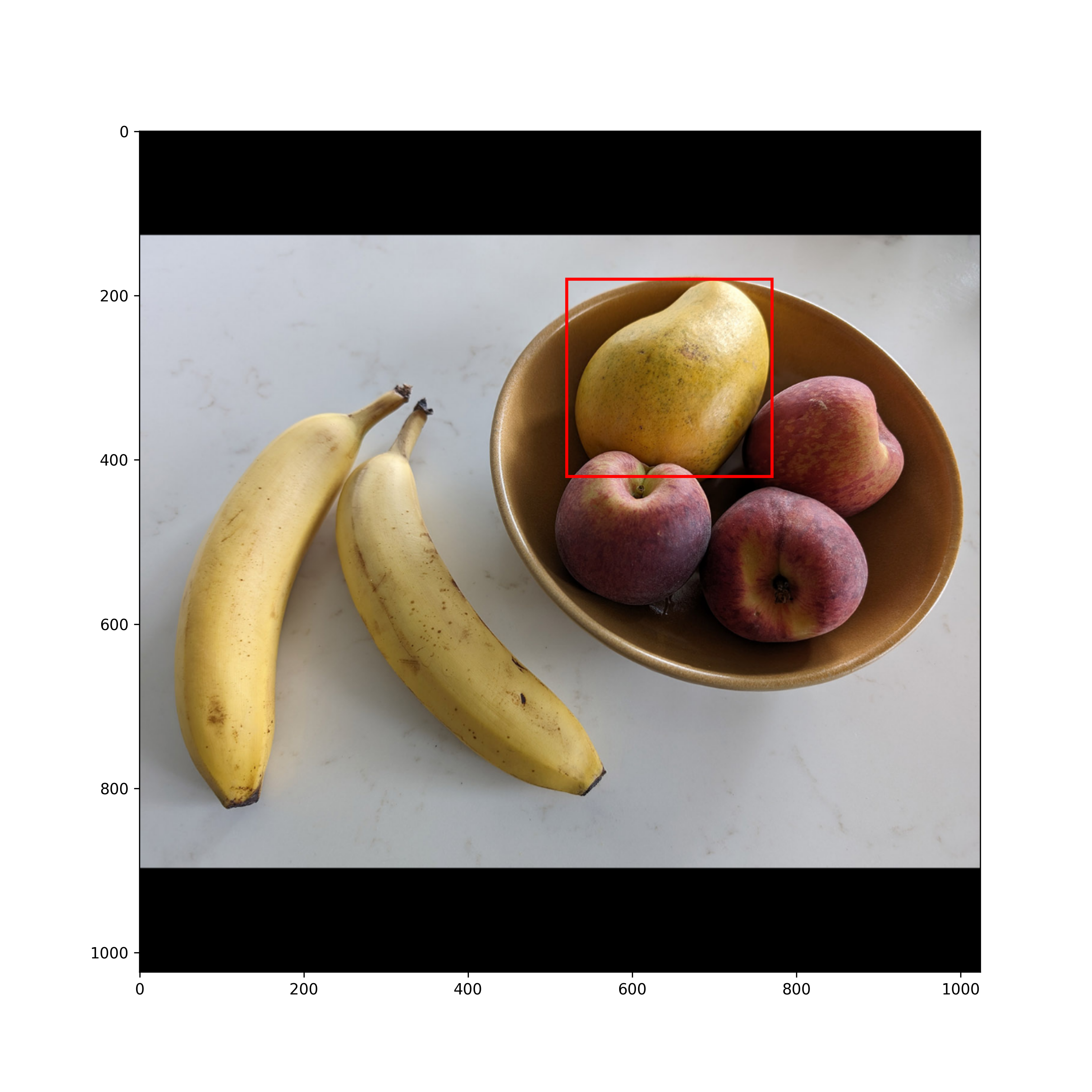
Prompting the model with a target box
Besides providing one or more target points, you can also provide boxes approximating the location of the object to segment. These boxes should be passed via the coordinates of their top-left and bottom-right corners. Here’s a box around the mango (see figure 11.14):
input_box = np.array(
    [
        # Top-left corner
        [520, 180],
        # Bottom-right corner
        [770, 420],
    ]
)

plt.figure(figsize=(10, 10))
show_image(image, plt.gca())
show_box(input_box, plt.gca())
plt.show()
Let’s prompt SAM with it (see figure 11.15):
outputs = model.predict(
    {
        "images": ops.expand_dims(image, axis=0),
        "boxes": ops.expand_dims(input_box, axis=(0, 1)),
    }
)
mask = get_mask(outputs, 0)
plt.figure(figsize=(10, 10))
show_image(image, plt.gca())
show_mask(mask, plt.gca())
show_box(input_box, plt.gca())
plt.show()
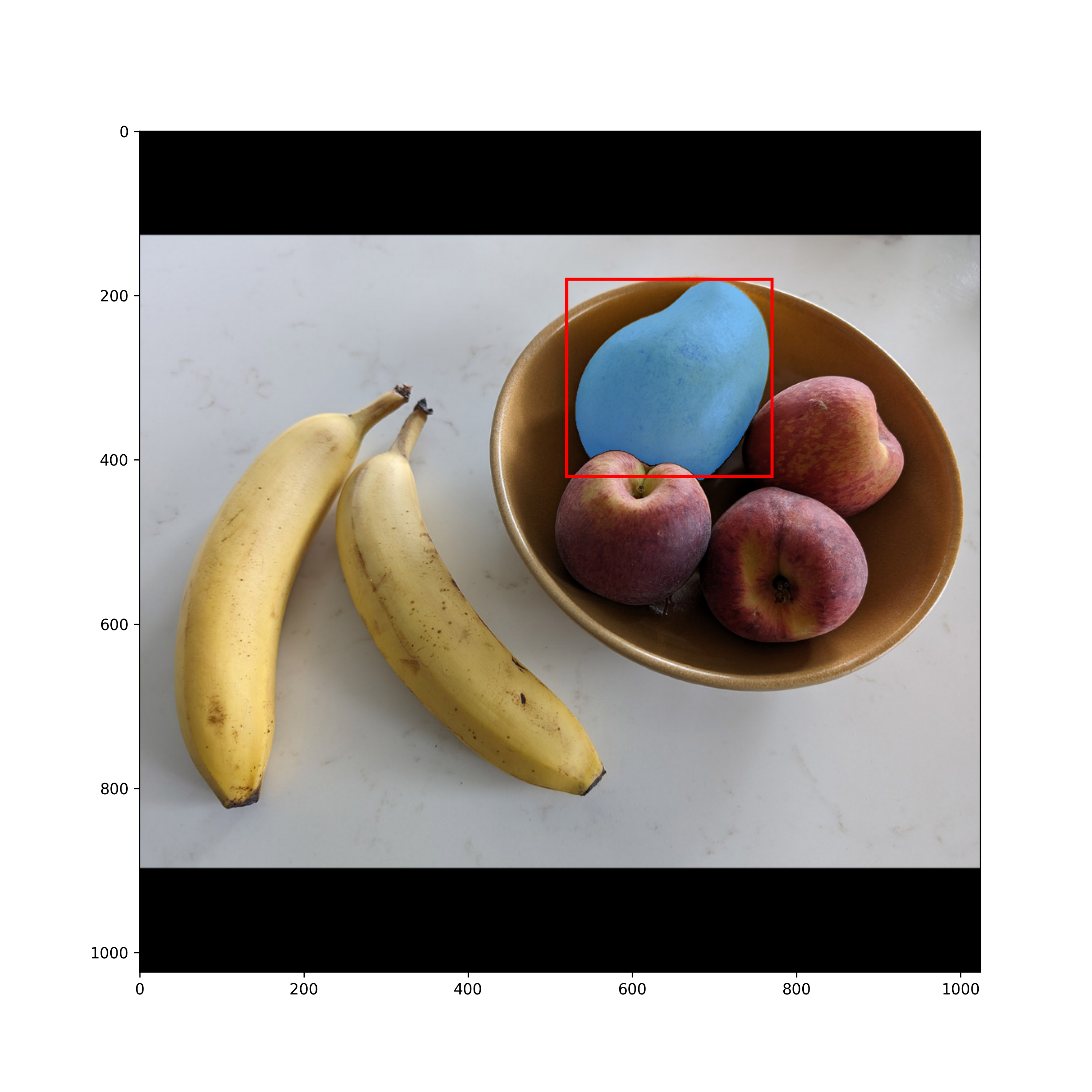
SAM can be a powerful tool to quickly create large datasets of images annotated with segmentation masks.
Summary
- Image segmentation is one of the main categories of computer vision tasks. It consists of computing segmentation masks that describe the contents of an image at the pixel level.
- To build your own segmentation model, use a stack of strided
Conv2Dlayers to “compress” the input image into a smaller feature map, followed by a stack of correspondingConv2DTransposelayers to “expand” the feature map into a segmentation mask the same size as the input image. - You can also use a pretrained segmentation model. Segment Anything, included in KerasHub, is a powerful model that supports image prompting, text prompting, point prompting, and box prompting.