


With the basics of text preprocessing and modeling covered in the previous chapter, this chapter will tackle some more involved language problems such as machine translation. We will build up a solid intuition for the Transformer model that powers products like ChatGPT and has helped trigger a wave of investment in natural language processing (NLP).
The language model
In the previous chapter, we learned how to convert text data to numeric inputs, and we used this numeric representation to classify movie reviews. However, text classification is, in many ways, a uniquely simple problem. We only need to output a single floating-point number for binary classification and, at worst, N numbers for N-way classification.
What about other text-based tasks like question answering or translation? For many real-world problems, we are interested in a model that can generate a text output for a given input. Just like we needed tokenizers and embeddings to help us handle text on the way in to a model, we must build up some techniques before we can produce text on the way out.
We don’t need to start from scratch here; we can continue to use the idea of an integer sequence as a natural numeric representation for text. In the previous chapter, we covered tokenizing a string, where we split inputs into tokens and map each token to an int. We can detokenize a sequence by proceeding in reverse — map ints back to string tokens and join them together. With this approach, our problem becomes building a model that can predict an integer sequence of tokens.
The simplest option to consider might be to train a direct classifier over the space of all possible output integer sequences, but some back-of-the-envelope math will quickly show this is intractable. With a vocabulary of 20,000 words, there are 20,000 ^ 4, or 160 quadrillion possible 4-word sequences, and fewer atoms in the universe than possible 20-word sequences. Attempting to represent every output sequence as a unique classifier output would overwhelm compute resources no matter how we design our model.
A practical approach for making such a prediction problem feasible is to build a
model that only predicts a single token output at a time. A language model
is a model that, in its simplest form, learns a straightforward but deep
probability distribution: p(token|past tokens). Given a sequence of all tokens
observed up to a point, a language model will attempt to output a probability
distribution over all possible tokens that could come next. A 20,000-word
vocabulary means the model needs only predict 20,000 outputs, but by
repeatedly predicting the next token, we will have built a model that can
generate a long sequence of text.
Let’s make this more concrete by building a simple language model that predicts the next character in a sequence of characters. We will train a small model that can output Shakespeare-like text.
Training a Shakespeare language model
To begin, we can download a collection of some of Shakespeare’s plays and sonnets.
import keras

filename = keras.utils.get_file(
    origin=(
        "https://storage.googleapis.com/download.tensorflow.org/"
        "data/shakespeare.txt"
    ),
)
shakespeare = open(filename, "r").read()
Let’s take a look at some of the data:
>>> shakespeare[:250]First Citizen: Before we proceed any further, hear me speak. All: Speak, speak. First Citizen: You are all resolved rather to die than to famish? All: Resolved. resolved. First Citizen: First, you know Caius Marcius is chief enemy to the people.
To build a language model from this input, we will need to massage our source text. First, we will split our data into equal-length chunks that we can batch and use for model training, much as we did for weather measurements in the timeseries chapter. Because we will be using a character-level tokenizer here, we can do this chunking directly on the string input. A 100-character string will map to a 100-integer sequence.
We will also split each input into two separate feature and label sequences, with each label sequence simply being the input sequence offset by a single character.
import tensorflow as tf

# The chunk size we will use during training. We only train on
# sequences of 100 characters at a time.
sequence_length = 100

def split_input(input, sequence_length):
    for i in range(0, len(input), sequence_length):
        yield input[i : i + sequence_length]

features = list(split_input(shakespeare[:-1], sequence_length))
labels = list(split_input(shakespeare[1:], sequence_length))
dataset = tf.data.Dataset.from_tensor_slices((features, labels))
Let’s look at an (x, y) input sample. Our label at each position in the
sequence is the next character in the sequence:
>>> x, y = next(dataset.as_numpy_iterator()) >>> x[:50], y[:50](b"First Citizen:\nBefore we proceed any further, hear", b"irst Citizen:\nBefore we proceed any further, hear ")
To map this input to a sequence of integers, we can again use the
TextVectorization layer we saw in the last chapter. To learn a character-level
vocabulary instead of a word-level vocabulary, we can change our split
argument. Rather than the default "whitespace" splitting, we instead split by
"character". We will do no standardization here — to keep things simple, we
will preserve case and pass punctuation through unaltered.
from keras import layers

tokenizer = layers.TextVectorization(
    standardize=None,
    split="character",
    output_sequence_length=sequence_length,
)
tokenizer.adapt(dataset.map(lambda text, labels: text))
TextVectorization layer
Let’s inspect the vocabulary:
>>> vocabulary_size = tokenizer.vocabulary_size() >>> vocabulary_size67
We need only 67 characters to handle the full source text.
Next, we can apply our tokenization layer to our input text. And finally, we can shuffle, batch, and cache our dataset so we don’t need to recompute it every epoch:
dataset = dataset.map(
    lambda features, labels: (tokenizer(features), tokenizer(labels)),
    num_parallel_calls=8,
)
training_data = dataset.shuffle(10_000).batch(64).cache()
With that, we are ready to start modeling.
To build our simple language model, we want to predict the probability of a
character given all past characters. Of all the modeling possibilities we have
seen so far in this book, an RNN is the most natural fit, as the recurrent state
of each cell allows the model to propagate information about past characters
when predicting the label of the current character. We can also use an Embedding, as we saw in the previous chapter, to embed each
input character as a unique 256-dimensional vector.
We will use only a single recurrent layer to keep this model small and easy to
train. Any recurrent layer would do here, but to keep things simple, we will use
a GRU, which is fast and has a simpler internal state than an LSTM.
embedding_dim = 256
hidden_dim = 1024

inputs = layers.Input(shape=(sequence_length,), dtype="int", name="token_ids")
x = layers.Embedding(vocabulary_size, embedding_dim)(inputs)
x = layers.GRU(hidden_dim, return_sequences=True)(x)
x = layers.Dropout(0.1)(x)
# Outputs a probability distribution over all potential tokens in our
# vocabulary
outputs = layers.Dense(vocabulary_size, activation="softmax")(x)
model = keras.Model(inputs, outputs)
Let’s take a look at our model summary:
>>> model.summary()Model: "functional" ┏━━━━━━━━━━━━━━━━━━━━━━━━━━━━━━━━━━━┳━━━━━━━━━━━━━━━━━━━━━━━━━━┳━━━━━━━━━━━━━━━┓ ┃ Layer (type) ┃ Output Shape ┃ Param # ┃ ┡━━━━━━━━━━━━━━━━━━━━━━━━━━━━━━━━━━━╇━━━━━━━━━━━━━━━━━━━━━━━━━━╇━━━━━━━━━━━━━━━┩ │ token_ids (InputLayer) │ (None, 100) │ 0 │ ├───────────────────────────────────┼──────────────────────────┼───────────────┤ │ embedding (Embedding) │ (None, 100, 256) │ 17,152 │ ├───────────────────────────────────┼──────────────────────────┼───────────────┤ │ gru (GRU) │ (None, 100, 1024) │ 3,938,304 │ ├───────────────────────────────────┼──────────────────────────┼───────────────┤ │ dropout (Dropout) │ (None, 100, 1024) │ 0 │ ├───────────────────────────────────┼──────────────────────────┼───────────────┤ │ dense (Dense) │ (None, 100, 67) │ 68,675 │ └───────────────────────────────────┴──────────────────────────┴───────────────┘ Total params: 4,024,131 (15.35 MB) Trainable params: 4,024,131 (15.35 MB) Non-trainable params: 0 (0.00 B)
This model outputs a softmax probability for every possible character in our
vocabulary, and we will compile() it with a crossentropy loss. Note that our
model is still training on a classification problem, it’s just that we will make
one classification prediction for every token in our sequence. For our batch of
64 samples with 100 characters each, we will predict 6,400 individual labels.
Loss and accuracy metrics reported by Keras during training will be averaged
first across each sequence and, second, across each batch.
Let’s go ahead and train our language model.
model.compile(
    optimizer="adam",
    loss="sparse_categorical_crossentropy",
    metrics=["sparse_categorical_accuracy"],
)
model.fit(training_data, epochs=20)
After 20 epochs, our model can eventually predict the next character in our input sequences around 70% of the time.
Generating Shakespeare
Now that we have trained a model that can predict the next individual tokens with some accuracy, we would like to use it to extrapolate an entire predicted sequence. We can do this by calling the model in a loop, where the model’s predicted output at one time step becomes the model’s input at the next time step. A model built for this kind of feedback loop is sometimes called an autoregressive model.
To run such a loop, we need to perform a slight surgery on the model we just
trained. During training, our model handled only a fixed sequence length of 100
tokens, and the GRU cell’s state was handled implicitly when calling the
layer. During generation, we would like to predict a single output token at a
time and explicitly output the state of the GRU’s cell. We need to propagate
that state, which contains all information the model has encoded about past
input characters, the next time we call the model.
Let’s make a model that handles a single input character at a time and allows explicitly passing the RNN state. Because this model will have the same computational structure, with slightly modified inputs and outputs, we can assign weights from one model to another.
# Creates a model that receives and outputs the RNN state
inputs = keras.Input(shape=(1,), dtype="int", name="token_ids")
input_state = keras.Input(shape=(hidden_dim,), name="state")

x = layers.Embedding(vocabulary_size, embedding_dim)(inputs)
x, output_state = layers.GRU(hidden_dim, return_state=True)(
    x, initial_state=input_state
)
outputs = layers.Dense(vocabulary_size, activation="softmax")(x)
generation_model = keras.Model(
    inputs=(inputs, input_state),
    outputs=(outputs, output_state),
)
# Copies the parameters from the original model
generation_model.set_weights(model.get_weights())
With this, we can call the model to predict an output sequence in a loop. Before we do, we will make explicit lookup tables so we switch from characters to integers and choose a prompt — a snippet of text we will feed as input to the model before we begin predicting new tokens:
tokens = tokenizer.get_vocabulary()
token_ids = range(vocabulary_size)
char_to_id = dict(zip(tokens, token_ids))
id_to_char = dict(zip(token_ids, tokens))

prompt = """
KING RICHARD III:
"""
To begin generation, we first need to “prime” the internal state of the GRU with our prompt. To do this, we will feed the prompt into the model one token at a time. This will compute the exact RNN state the model would see if this prompt had been encountered during training.
When we feed the very last character of the prompt into the model, our state output will capture information about the entire prompt sequence. We can save the final output prediction to later select the first character of our generated response.
input_ids = [char_to_id[c] for c in prompt]
state = keras.ops.zeros(shape=(1, hidden_dim))
for token_id in input_ids:
    inputs = keras.ops.expand_dims([token_id], axis=0)
    # Feeds the prompt character by character to update state
    predictions, state = generation_model.predict((inputs, state), verbose=0)
Now we are ready to let the model predict a new output sequence. In a loop, up to a desired length, we will continually select the most likely next character predicted by the model, feed that to the model, and persist the new RNN state. In this way, we can predict an entire sequence, a token at time.
import numpy as np

generated_ids = []
max_length = 250
# Generates characters one by one, computing a new state each iteration
for i in range(max_length):
    # The next character is the output index with the highest
    # probability.
    next_char = int(np.argmax(predictions, axis=-1)[0])
    generated_ids.append(next_char)
    inputs = keras.ops.expand_dims([next_char], axis=0)
    predictions, state = generation_model.predict((inputs, state), verbose=0)
Let’s convert our output integer sequence to a string to see what the model predicted. To detokenize our input, we simply map all token IDs to strings and join them together:
output = "".join([id_to_char[token_id] for token_id in generated_ids])
print(prompt + output)
We get the following output:
KING RICHARD III:
Stay, men! hear me speak.

FRIAR LAURENCE:
Thou wouldst have done thee here that he hath made for them?

BUCKINGHAM:
What straight shall stop his dismal threatening son,
Thou bear them both. Here comes the king;
Though I be good to put a wife to him,
We have yet to produce the next great tragedy, but this is not terrible for two minutes of training on a minimal dataset. The goal of this toy example is to show the power of the language model setup. We trained the model on the narrow problem of guessing a single character at a time but still use it for a much broader problem, generating an open-ended, Shakespearean-like text response.
It’s important to notice that this training setup only works because a recurrent
neural network only passes information forward in the sequence. If you’d like,
try replacing the GRU layer with a Bidirectional(GRU(...)). The
training accuracy will zoom to above 99% immediately, and generation will stop
working entirely. During training, our model sees the entire sequence each train
step. If we “cheat” by letting information from the next token in the sequence
affect the current token’s prediction, we’ve made our problem trivially easy.
This language modeling setup is fundamental to countless problems in the
text domain. It is also somewhat unique compared to other modeling problems we
have seen so far in this book. We cannot simply call model.predict() to get
the desired output. There is an entire loop, and a nontrivial amount of logic,
that exists only at inference time! The looping of state in the RNN cell happens
for both training and inference, but at no point during training do we feed a
model’s predicted labels back into itself as input.
Sequence-to-sequence learning
Let’s take the language model idea and extend it to tackle an important problem — machine translation. Translation belongs to a class of modeling problems often called sequence-to-sequence modeling (or seq2seq if you are trying to save keystrokes). We seek to build a model that can take in a source text as a fixed input sequence and generate the translated text sequence as a result. Question answering is another classic sequence-to-sequence problem.
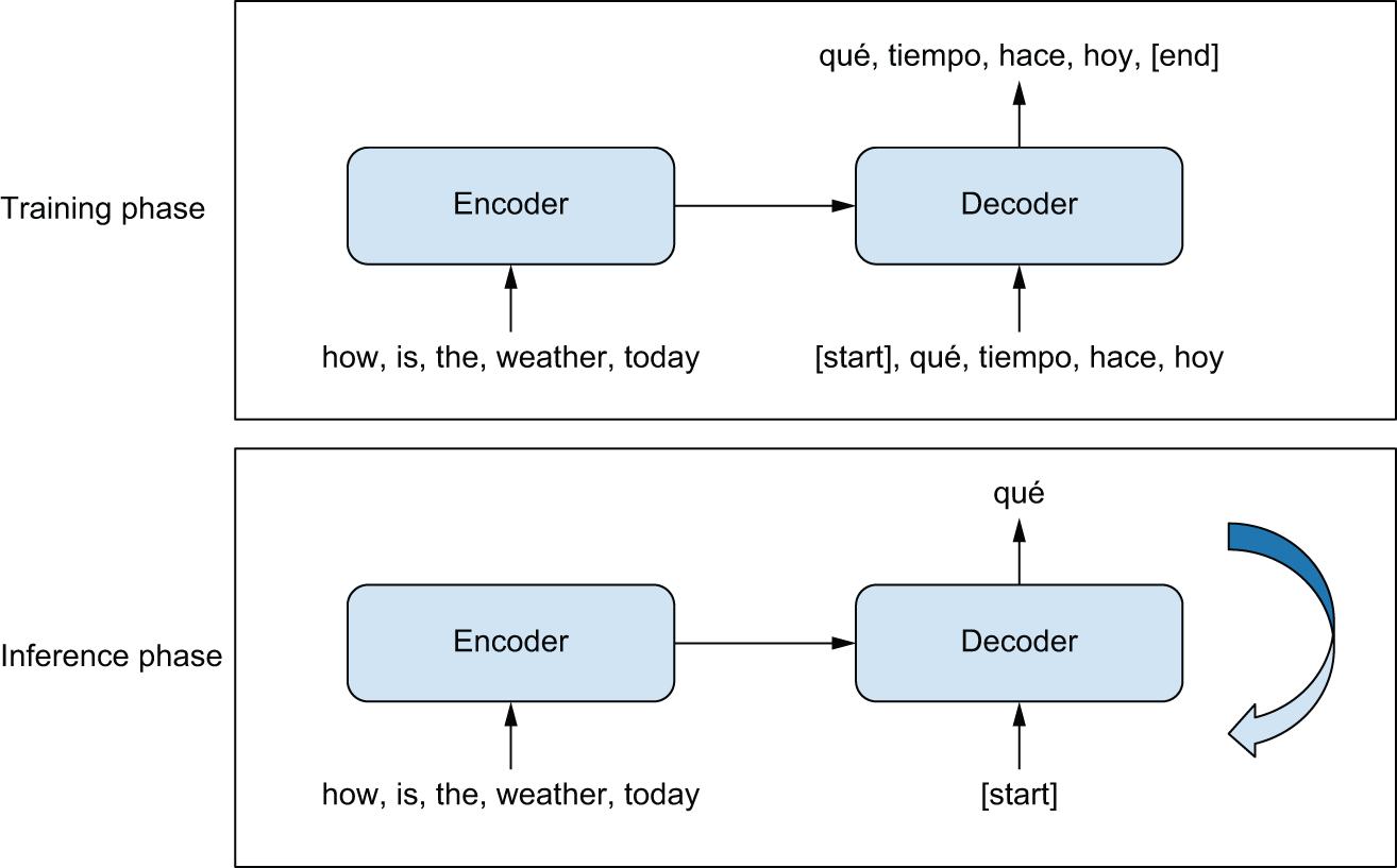
The general template behind sequence-to-sequence models is described in figure 15.1. During training, the following happens:
- An encoder model turns the source sequence into an intermediate representation.
- A decoder is trained using the language modeling setup we saw previously. It will recursively predict the next token in the target sequence by looking at all previous target tokens and our encoder’s representation of the source sequence.
During inference, we don’t have access to the target sequence — we’re trying to predict it from scratch. We will generate it one token at a time, just as we did with our Shakespeare generator:
- We obtain the encoded source sequence from the encoder.
- The decoder starts by looking at the encoded source sequence as well as an
initial “seed” token (such as the string
"[start]") and uses them to predict the first real token in the sequence. - The predicted sequence so far is fed back into the decoder, in a loop, until
it generates a stop token (such as the string
"[end]").
Let’s build a sequence-to-sequence translation model.
English-to-Spanish translation
We’ll be working with an English-to-Spanish translation dataset. Let’s download it:
import pathlib

zip_path = keras.utils.get_file(
    origin=(
        "http://storage.googleapis.com/download.tensorflow.org/data/spa-eng.zip"
    ),
    fname="spa-eng",
    extract=True,
)
text_path = pathlib.Path(zip_path) / "spa-eng" / "spa.txt"
The text file contains one example per line: an English sentence, followed by a tab character, followed by the corresponding Spanish sentence. Let’s parse this file:
with open(text_path) as f:
    lines = f.read().split("\n")[:-1]
text_pairs = []
for line in lines:
    english, spanish = line.split("\t")
    spanish = "[start] " + spanish + " [end]"
    text_pairs.append((english, spanish))
Our text_pairs look like this:
>>> import random >>> random.choice(text_pairs)("Who is in this room?", "[start] ¿Quién está en esta habitación? [end]")
Let’s shuffle them and split them into the usual training, validation, and test sets:
import random

random.shuffle(text_pairs)
val_samples = int(0.15 * len(text_pairs))
train_samples = len(text_pairs) - 2 * val_samples
train_pairs = text_pairs[:train_samples]
val_pairs = text_pairs[train_samples : train_samples + val_samples]
test_pairs = text_pairs[train_samples + val_samples :]
Next, let’s prepare two separate TextVectorization layers: one for English and
one for Spanish. We’re going to need to customize the way strings are
preprocessed:
- We need to preserve the
"[start]"and"[end]"tokens that we’ve inserted. By default, the characters[and]would be stripped, but we want to keep them around so we can distinguish the word"start"from the start token"[start]". - Punctuation is different from language to language! In the Spanish
TextVectorizationlayer, if we’re going to strip punctuation characters, we need to also strip the character¿.
Note that for a non-toy translation model, we would treat punctuation characters as separate tokens rather than stripping them since we would want to be able to generate correctly punctuated sentences. In our case, for simplicity, we’ll get rid of all punctuation.
import string
import re

strip_chars = string.punctuation + "¿"
strip_chars = strip_chars.replace("[", "")
strip_chars = strip_chars.replace("]", "")

def custom_standardization(input_string):
    lowercase = tf.strings.lower(input_string)
    return tf.strings.regex_replace(
        lowercase, f"[{re.escape(strip_chars)}]", ""
    )

vocab_size = 15000
sequence_length = 20

english_tokenizer = layers.TextVectorization(
    max_tokens=vocab_size,
    output_mode="int",
    output_sequence_length=sequence_length,
)
spanish_tokenizer = layers.TextVectorization(
    max_tokens=vocab_size,
    output_mode="int",
    output_sequence_length=sequence_length + 1,
    standardize=custom_standardization,
)
train_english_texts = [pair[0] for pair in train_pairs]
train_spanish_texts = [pair[1] for pair in train_pairs]
english_tokenizer.adapt(train_english_texts)
spanish_tokenizer.adapt(train_spanish_texts)
Finally, we can turn our data into a tf.data pipeline. We want it to return a
tuple (inputs, target, sample_weights) where inputs is a dict with two keys,
"english" (the tokenized English sentence) and "spanish" (the tokenized
Spanish sentence), and target is the Spanish sentence offset by one step
ahead. sample_weights here will be used to tell Keras which labels to use when
calculating our loss and metrics. Our output translations are not all equal in
length, and some of our label sequences will be padded with zeros. We only care
about predictions for non-zero labels that represent actual translated text.
This matches the “off by one” label set up in the generation model we just built, with the addition of the fixed encoder inputs, which will be handled separately in our model.
batch_size = 64

def format_dataset(eng, spa):
    eng = english_tokenizer(eng)
    spa = spanish_tokenizer(spa)
    features = {"english": eng, "spanish": spa[:, :-1]}
    labels = spa[:, 1:]
    sample_weights = labels != 0
    return features, labels, sample_weights

def make_dataset(pairs):
    eng_texts, spa_texts = zip(*pairs)
    eng_texts = list(eng_texts)
    spa_texts = list(spa_texts)
    dataset = tf.data.Dataset.from_tensor_slices((eng_texts, spa_texts))
    dataset = dataset.batch(batch_size)
    dataset = dataset.map(format_dataset, num_parallel_calls=4)
    return dataset.shuffle(2048).cache()

train_ds = make_dataset(train_pairs)
val_ds = make_dataset(val_pairs)
Here’s what our dataset outputs look like:
>>> inputs, targets, sample_weights = next(iter(train_ds)) >>> print(inputs["english"].shape)(64, 20)>>> print(inputs["spanish"].shape)(64, 20)>>> print(targets.shape)(64, 20)>>> print(sample_weights.shape)(64, 20)
The data is now ready — time to build some models.
Sequence-to-sequence learning with RNNs
Before we try the twin encoder/decoder setup we previously mentioned, let’s think through simpler options. The easiest, naive way to use RNNs to turn one sequence into another is to keep the output of the RNN at each time step and predict an output token from it. In Keras, it would look like this:
inputs = keras.Input(shape=(sequence_length,), dtype="int32")
x = layers.Embedding(input_dim=vocab_size, output_dim=128)(inputs)
x = layers.LSTM(32, return_sequences=True)(x)
outputs = layers.Dense(vocab_size, activation="softmax")(x)
model = keras.Model(inputs, outputs)
However, there is a critical issue with this approach. Due to the step-by-step
nature of RNNs, the model will only look at tokens 0...N in the source
sequence to predict token N in the target sequence. Consider translating the
sentence, “I will bring the bag to you.” In Spanish, that would be “Te traeré
la bolsa,” where “Te,” the first word of the translation, corresponds to “you”
in the English source text. There’s simply no way to output the first word of
the translation without seeing the last word of the source English text!
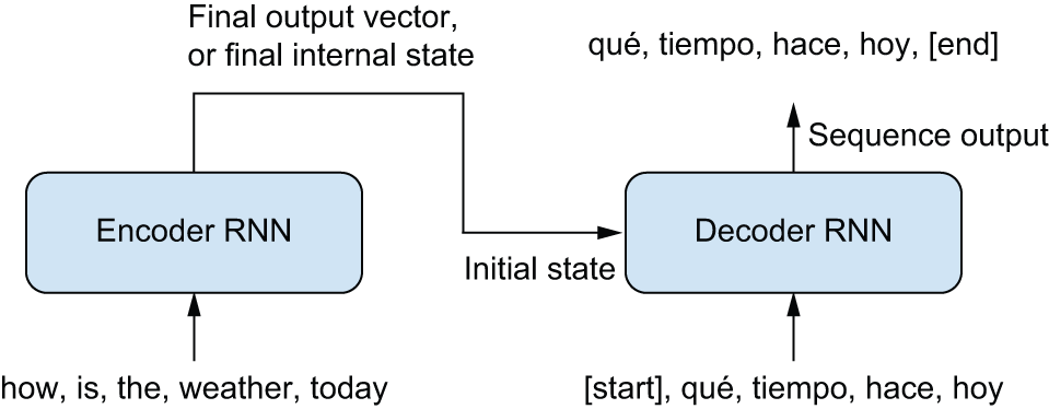
If you’re a human translator, you’d start by reading the entire source sentence before beginning to translate it. This is especially important if you’re dealing with languages with wildly different word ordering. And that’s precisely what standard sequence-to-sequence models do. In a proper sequence-to-sequence setup (see figure 15.2), you would first use an encoder RNN to turn the entire source sequence into a single representation of the source text. This could be the last output of the RNN or, alternatively, its final internal state vectors. We can use this representation as the initial state of a decoder RNN in the language model setup instead of an initial state of zeros, which we used in our Shakespeare generator. This decoder learns to predict the next word of the Spanish translation given the current word of the translation, with all information about the English sequence coming from that initial RNN state.
Let’s implement this in Keras, with GRU-based encoders and decoders. We can
start with just the encoder. Since we will not actually be predicting tokens in
the encoder sequence, we don’t have to worry about “cheating” by letting the model
pass information from the end of the sequence to positions at the beginning.
In fact, this is a good idea, as we want a rich representation of the source
sequence. We can achieve this with a Bidirectional layer.
embed_dim = 256
hidden_dim = 1024

source = keras.Input(shape=(None,), dtype="int32", name="english")
x = layers.Embedding(vocab_size, embed_dim, mask_zero=True)(source)
rnn_layer = layers.GRU(hidden_dim)
rnn_layer = layers.Bidirectional(rnn_layer, merge_mode="sum")
encoder_output = rnn_layer(x)
Next, let’s add the decoder — a simple GRU layer that takes as its initial state
the encoded source sentence. On top of it, we add a Dense layer that produces
a probability distribution over the Spanish vocabulary for each output step.
Here, we want to predict the next tokens based only on what came before, so a
Bidirectional RNN would break training by making the loss function trivially
easy.
target = keras.Input(shape=(None,), dtype="int32", name="spanish")
x = layers.Embedding(vocab_size, embed_dim, mask_zero=True)(target)
rnn_layer = layers.GRU(hidden_dim, return_sequences=True)
x = rnn_layer(x, initial_state=encoder_output)
x = layers.Dropout(0.5)(x)
# Predicts the next word of the translation, given the current word
target_predictions = layers.Dense(vocab_size, activation="softmax")(x)
seq2seq_rnn = keras.Model([source, target], target_predictions)
Let’s take a look at the seq2seq model in full:
>>> seq2seq_rnn.summary()Model: "functional_1" ┏━━━━━━━━━━━━━━━━━━━━━━━┳━━━━━━━━━━━━━━━━━━━┳━━━━━━━━━━━━━┳━━━━━━━━━━━━━━━━━━━━┓ ┃ Layer (type) ┃ Output Shape ┃ Param # ┃ Connected to ┃ ┡━━━━━━━━━━━━━━━━━━━━━━━╇━━━━━━━━━━━━━━━━━━━╇━━━━━━━━━━━━━╇━━━━━━━━━━━━━━━━━━━━┩ │ english (InputLayer) │ (None, None) │ 0 │ - │ ├───────────────────────┼───────────────────┼─────────────┼────────────────────┤ │ spanish (InputLayer) │ (None, None) │ 0 │ - │ ├───────────────────────┼───────────────────┼─────────────┼────────────────────┤ │ embedding_1 │ (None, None, 256) │ 3,840,000 │ english[0][0] │ │ (Embedding) │ │ │ │ ├───────────────────────┼───────────────────┼─────────────┼────────────────────┤ │ not_equal (NotEqual) │ (None, None) │ 0 │ english[0][0] │ ├───────────────────────┼───────────────────┼─────────────┼────────────────────┤ │ embedding_2 │ (None, None, 256) │ 3,840,000 │ spanish[0][0] │ │ (Embedding) │ │ │ │ ├───────────────────────┼───────────────────┼─────────────┼────────────────────┤ │ bidirectional │ (None, 1024) │ 7,876,608 │ embedding_1[0][0], │ │ (Bidirectional) │ │ │ not_equal[0][0] │ ├───────────────────────┼───────────────────┼─────────────┼────────────────────┤ │ gru_2 (GRU) │ (None, None, │ 3,938,304 │ embedding_2[0][0], │ │ │ 1024) │ │ bidirectional[0][… │ ├───────────────────────┼───────────────────┼─────────────┼────────────────────┤ │ dropout_1 (Dropout) │ (None, None, │ 0 │ gru_2[0][0] │ │ │ 1024) │ │ │ ├───────────────────────┼───────────────────┼─────────────┼────────────────────┤ │ dense_1 (Dense) │ (None, None, │ 15,375,000 │ dropout_1[0][0] │ │ │ 15000) │ │ │ └───────────────────────┴───────────────────┴─────────────┴────────────────────┘ Total params: 34,869,912 (133.02 MB) Trainable params: 34,869,912 (133.02 MB) Non-trainable params: 0 (0.00 B)
Our model and data are both ready. We can now begin training our translation model:
seq2seq_rnn.compile(
    optimizer="adam",
    loss="sparse_categorical_crossentropy",
    weighted_metrics=["accuracy"],
)
seq2seq_rnn.fit(train_ds, epochs=15, validation_data=val_ds)
We picked accuracy as a crude way to monitor validation set performance during
training. We get to 65% accuracy: on average, the model correctly predicts the
next word in the Spanish sentence 65% of the time. However, in practice,
next-token accuracy isn’t a great metric for machine translation models, in
particular because it makes the assumption that the correct target tokens from
0 to N are already known when predicting token N + 1. In reality, during
inference, you’re generating the target sentence from scratch, and you can’t
rely on previously generated tokens being 100% correct. When working on a
real-world machine translation system, metrics must be more carefully designed.
There are standard metrics, such as a BLEU score, that measure the similarity
of the machine-translated text to a set of high-quality reference translations
and can tolerate slightly misaligned sequences.
At last, let’s use our model for inference. We’ll pick a few sentences in the
test set and check how our model translates them. We’ll start from the seed
token "[start]" and feed it into the decoder model, together with the
encoded English source sentence. We’ll retrieve a next-token prediction, and
we’ll re-inject it into the decoder repeatedly, sampling one new target token at
each iteration, until we get to "[end]" or reach the maximum sentence length.
import numpy as np

spa_vocab = spanish_tokenizer.get_vocabulary()
spa_index_lookup = dict(zip(range(len(spa_vocab)), spa_vocab))

def generate_translation(input_sentence):
    tokenized_input_sentence = english_tokenizer([input_sentence])
    decoded_sentence = "[start]"
    for i in range(sequence_length):
        tokenized_target_sentence = spanish_tokenizer([decoded_sentence])
        inputs = [tokenized_input_sentence, tokenized_target_sentence]
        next_token_predictions = seq2seq_rnn.predict(inputs, verbose=0)
        sampled_token_index = np.argmax(next_token_predictions[0, i, :])
        sampled_token = spa_index_lookup[sampled_token_index]
        decoded_sentence += " " + sampled_token
        if sampled_token == "[end]":
            break
    return decoded_sentence

test_eng_texts = [pair[0] for pair in test_pairs]
for _ in range(5):
    input_sentence = random.choice(test_eng_texts)
    print("-")
    print(input_sentence)
    print(generate_translation(input_sentence))
The exact translations will vary from run to run, as the final model weights will depend on the random initializations of our weights and the random shuffling of our input data. Here’s what we got:
-
You know that.
[start] tú lo sabes [end]
-
"Thanks." "You're welcome."
[start] gracias tú [UNK] [end]
-
The prisoner was set free yesterday.
[start] el plan fue ayer a un atasco [end]
-
I will tell you tomorrow.
[start] te lo voy mañana a decir [end]
-
I think they're happy.
[start] yo creo que son felices [end]
Our model works decently well for a toy model, although it still makes many basic mistakes.
Note that this inference setup, while very simple, is inefficient, since we reprocess the entire source sentence and the entire generated target sentence every time we sample a new word. In a practical application, you’d want to be careful not to recompute any state that has not changed. All we really need to predict a new token in the decoder is the current token and the previous RNN state, which we could cache before each loop iteration.
There are many ways this toy model could be improved. We could use a deep stack
of recurrent layers for both the encoder and the decoder, we could try other RNN
layers like LSTM, and so on. Beyond such tweaks, however, the RNN approach to
sequence-to-sequence learning has a few fundamental limitations:
- The source sequence representation has to be held entirely in the encoder state vector, which significantly limits the size and complexity of the sentences you can translate.
- RNNs have trouble dealing with very long sequences since they tend to progressively forget about the past — by the time you’ve reached the 100th token in either sequence, little information remains about the start of the sequence.
Recurrent neural networks dominated sequence-to-sequence learning in the
mid-2010s. Google Translate circa 2017 was powered by a stack of seven large
LSTM layers in a setup similar to what we just created. However, these
limitations of RNNs eventually led to researchers developing a new style of
sequence model, called the Transformer.
The Transformer architecture
In 2017, Vaswani et al. introduced the Transformer architecture in the seminal paper “Attention Is All You Need.”[1] The authors were working on translation systems like the one we just built, and the critical discovery is right in the title. As it turned out, a simple mechanism called attention can be used to construct powerful sequence models that don’t feature recurrent layers at all. The idea of attention was not new and had been used in NLP systems for a couple of years when they published. But the idea that attention was so useful it could be the only mechanism used to pass information across a sequence was quite surprising at the time.
This finding unleashed nothing short of a revolution in natural language processing — and beyond. Attention has fast become one of the most influential ideas in deep learning. In this section, you’ll get an in-depth explanation of how it works and why it has proven so effective for sequence modeling. We’ll then use attention to rebuild our English-to-Spanish translation model.
So, with all that as build-up, what exactly is attention? And how does it offer a replacement for the recurrent neural networks we have used so far?
Attention was actually developed as a way to augment an RNN model like the one we just built. Researchers noticed that while RNNs excelled at modeling dependencies in a local neighborhood, they struggled with recall as sequences got longer. Say you were building a system to answer questions about a source document. If the document length got too long, RNN results would get plain bad, a far cry from human performance.
As a thought experiment, imagine using this book to build a weather prediction model. If you had enough time, you might read the entire book cover to cover, but when you actually implemented your model, you would pay special attention to just the timeseries chapters. Even within a chapter, you might find specific code samples and explanations you would refer to often. On the other hand, you would not be particularly worried about the details of image convolutions as you worked on your code. The overall word count of this book is well over 100,000, far beyond any sequence length we have tackled, but humans can be selective and contextual in how we pull information from text.
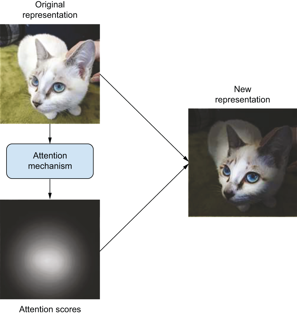
RNNs, on the other hand, lack any mechanism to refer back to a previous section of a sequence directly. All information must, by design, be passed through an RNN cell’s internal state in a loop, through every position in a sequence. It’s a bit like finishing this book, closing it, and trying to implement that weather prediction model entirely from memory. The idea with attention is to build a mechanism by which a neural network can give more weight to some part of a sequence and less weight to others contextually, depending on the current input being processed (figure 15.3).
Dot-product attention
Let’s revisit our translation RNN and try to add the notion of selective
attention. Consider predicting just a single token. After passing the source
and target sequences through our GRU layers, we will have a vector
representing the target token we are about to predict and a sequence of vectors
representing each word in the source text.
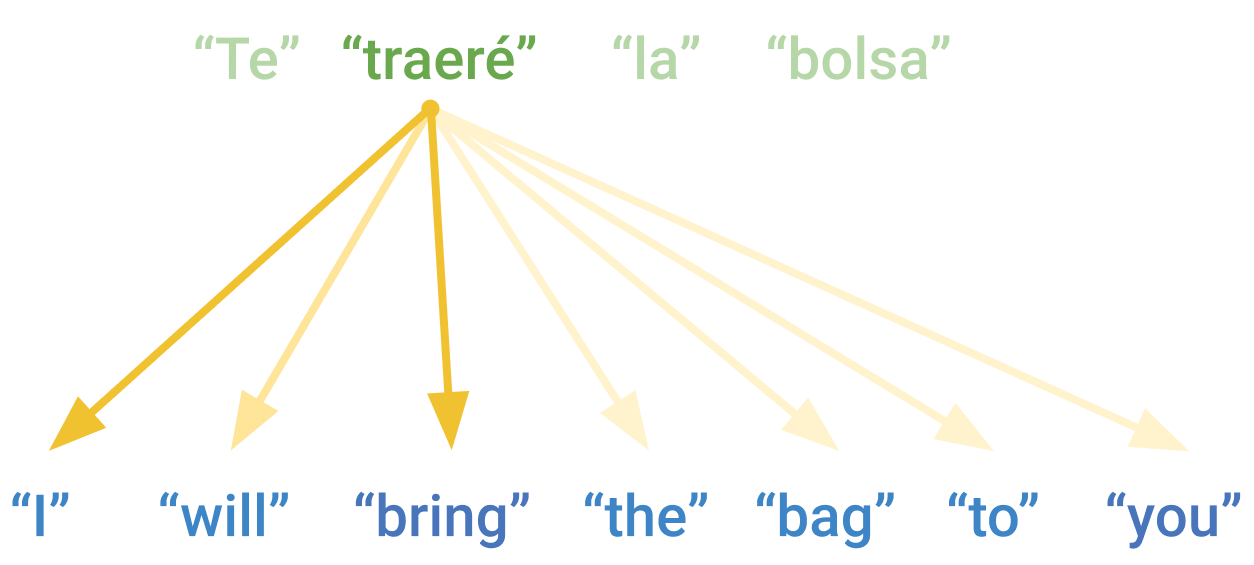
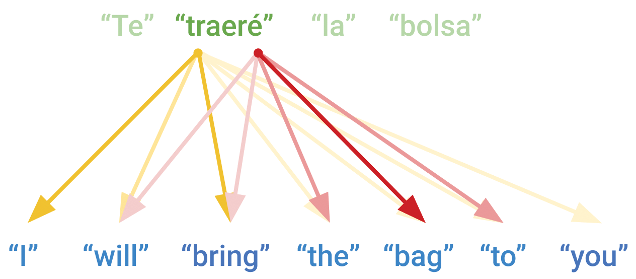
With attention, our goal is to give the model a way to score every single
vector in our source sequence based on its relevance to the current word we
are trying to predict (figure 15.4). If the vector representation of a source token has a high
score, we consider it particularly important; if not, we care less about it. For
now, let’s assume we have this function score(target_vector, source_vector).
For attention to work well, we want to avoid passing information about important
tokens through a loop potentially as long as our combined source and target
sequence length — this is where RNNs start to fail. A simple way to do this is to
take a weighted sum of all the source vectors based on this score we will
compute. It would also be convenient if the sum of all attention scores for a
given target were 1, as this would give our weighted sum a predictable
magnitude. We can achieve this by running the scores through a softmax function —
something like this, in NumPy pseudocode:
scores = [score(target, source) for source in sources]
scores = softmax(scores)
combined = np.sum(scores * sources)
But how should we compute this relevance score? When researchers first worked with attention, this question was a big topic of inquiry. It turns out that one of the most straightforward approaches is best. We can use a dot-product as a simple measure of the distance between target and source vectors. If the source and target vectors are close together, we assume that means the source token is relevant to our prediction. At the end of this chapter, we will examine why this assumption makes intuitive sense.
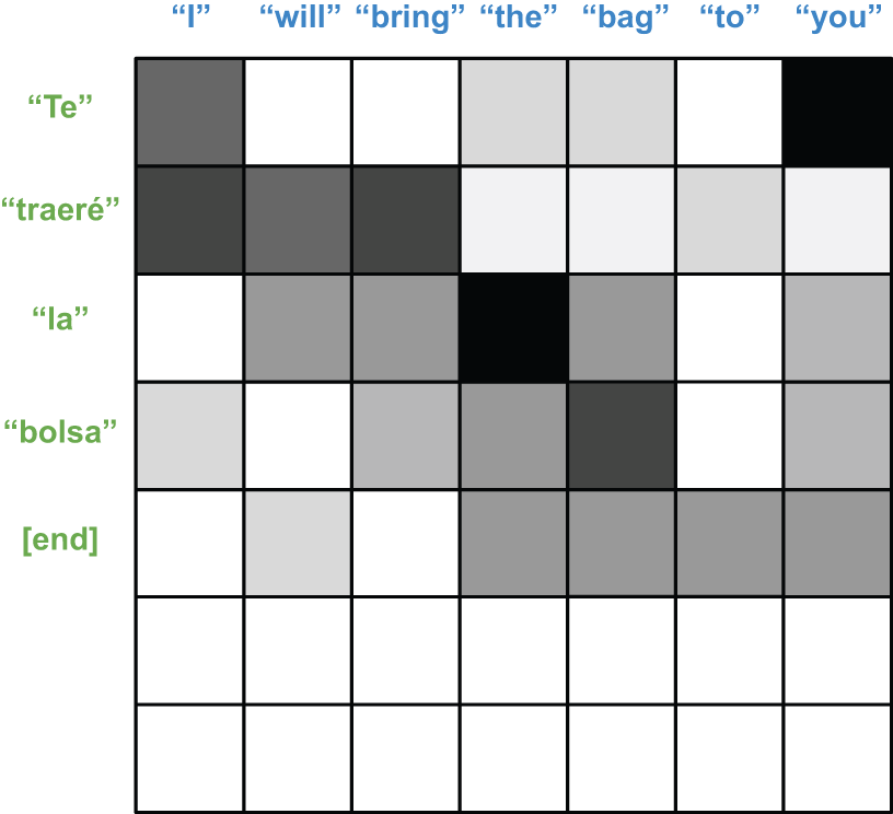
Let’s update our pseudocode. We can make our snippet more complete by handling
the entire target sequence at once — it will be equivalent to running our
previous snippet in a loop for each token in the target sequence. When both
target and source are sequences, the attention scores will be a matrix. Each
row represents how much a target word will value a source word in the weighted
sum (see figure 15.5). We will use the Einsum notation as a convenient way to
write the dot-product and weighted sum:
def dot_product_attention(target, source):
    # Takes the dot-product between all target and source vectors,
    # where b = batch size, t = target length, s = source length, and d
    # = vector size
    scores = np.einsum("btd,bsd->bts", target, source)
    scores = softmax(scores, axis=-1)
    # Computes a weighted sum of all source vectors for each target
    # vector
    return np.einsum("bts,bsd->btd", scores, source)

dot_product_attention(target, source)
We can make the hypothesis space of this attention mechanism much richer if we
give the model parameters to control the attention score. If we project both
source and target vectors with Dense layers, the model can find a good
shared space where source vectors are close to target vectors if they help the
overall prediction quality. Similarly, we should allow the model to project the
source vectors into an entirely separate space before they are combined and once
again after the summation.
We can also adopt a slightly different naming for inputs that has become
standard in the field. What we just wrote is roughly summarized as
sum(score(target, source) * source). We will write this equivalently with
different input names as sum(score(query, key) * value). This three-argument
version is more general — in rare cases, you might not want to use the same
vector to score your source inputs as you use to sum your source inputs.
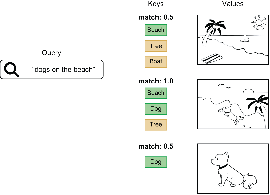
The terminology comes from search engines and recommender systems. Imagine a search tool to look up photos in a database — the “query” is your search term, the “keys” are photo tags you use to match with the query, and finally, the “values” are the photos themselves (figure 15.6). The attention mechanism we are building is roughly analogous to this sort of lookup.
Let’s update our pseudocode, so we have a parameterized attention using our new terminology:
query_dense = layers.Dense(dim)
key_dense = layers.Dense(dim)
value_dense = layers.Dense(dim)
output_dense = layers.Dense(dim)

def parameterized_attention(query, key, value):
    query = query_dense(query)
    key = key_dense(key)
    value = value_dense(value)
    scores = np.einsum("btd,bsd->bts", query, key)
    scores = softmax(scores, axis=-1)
    outputs = np.einsum("bts,bsd->btd", scores, value)
    return output_dense(outputs)

parameterized_attention(query=target, key=source, value=source)
This block is a perfectly functional attention mechanism! We just wrote a function that will allow the model to pull information from anywhere in the source sequence, contextually, depending on the target word we are decoding.
The “Attention is all you need” authors made two more changes to our mechanism through trial and error. The first is a simple scaling factor. When input vectors get long, the dot-product scores can get quite large, which can affect the stability of our softmax gradients. The fix is simple: we can scale down our softmax scores slightly. Scaling by the square root of the vector length works well for any vector size.
The other has to do with the expressivity of the attention mechanism. The softmax sum we are doing is powerful — it allows a direct connection across distant parts of a sequence. But the summation is also blunt: if the model tries to attend to too many tokens at once, the interesting features of individual source tokens will get “washed out” in the combined representation. A simple trick that works well is to do this attention operation several times for the same sequence, with several different attention heads running the same computation with different parameters:
query_dense = [layers.Dense(head_dim) for i in range(num_heads)]
key_dense = [layers.Dense(head_dim) for i in range(num_heads)]
value_dense = [layers.Dense(head_dim) for i in range(num_heads)]
output_dense = layers.Dense(head_dim * num_heads)

def multi_head_attention(query, key, value):
    head_outputs = []
    for i in range(num_heads):
        query = query_dense[i](query)
        key = key_dense[i](key)
        value = value_dense[i](value)
        scores = np.einsum("btd,bsd->bts", target, source)
        scores = softmax(scores / math.sqrt(head_dim), axis=-1)
        head_output = np.einsum("bts,bsd->btd", scores, source)
        head_outputs.append(head_output)
    outputs = ops.concatenate(head_outputs, axis=-1)
    return output_dense(outputs)

multi_head_attention(query=target, key=source, value=source)
By projecting the query and key differently, one head might learn to match the subject of the source sentence, while another head might attend to punctuation. This multi-headed attention avoids the limitation of needing to combine the entire source sequence with a single softmax sum (figure 15.7).
Of course, in practice, you would want to write this code as a reusable layer.
Here, Keras has you covered. We can recreate our previous code with the
MultiHeadAttention layer as follows:
multi_head_attention = keras.layers.MultiHeadAttention(
    num_heads=num_heads,
    head_dim=head_dim,
)
multi_head_attention(query=target, key=source, value=source)
Transformer encoder block
One way to use the MultiHeadAttention layer would be to add it to our existing
RNN translation model. We could pass the sequence output from our encoder and
decoder into an attention layer and use its output to update our target sequence
before prediction. Attention would allow the model to handle long-range
dependencies in text that the GRU layer will struggle with. This does, in
fact, improve an RNN model’s capabilities and is how attention was first used in
the mid-2010s.
However, the authors of “Attention is all you need” realized you could go further and use attention as a general mechanism for handling all sequence data in a model. Although so far we have only looked at attention as a way to handle information passing between two sequences, you could also use attention as a way to let a sequence attend to itself:
multi_head_attention(key=source, value=source, query=source)
This is called self-attention, and it is quite powerful. With self-attention, each token can attend to every token in its own sequence, including itself, allowing the model to learn a representation of the word in context.
Consider an example sentence: “The train left the station on time.” Now, consider one word in the sentence: “station.” What kind of station are we talking about? Could it be a radio station? Maybe the International Space Station? With self-attention, the model could learn to give a high attention score to the pair of “station” and “train,” summing the vector used to represent “train” into the representation of the word “station.”
Self-attention gives the model an effective way to go from representing a word
in a vacuum to representing a word conditioned on all other tokens that appear
in the sequence. This sounds a lot like what an RNN is supposed to do. Can we
just go ahead and replace our RNN layers with MultiHeadAttention?
Almost! But not quite; we still need an essential ingredient for any deep neural
network — a nonlinear activation function. The MultiHeadAttention layer
combines linear projections of every element in a source sequence, but that’s
it. In a sense, it’s a very expressive pooling operation. Consider, in the
extreme case, a token length of one. In this case, the attention score matrix is
always a single one, and the entire layer boils down to a linear projection of
the source sequence, with no nonlinearities. You could stack 100 attention
layers together and still be able to simplify the entire computation to a single
matrix multiplication! That’s a real problem with the expressiveness of our
model.
At some point, all recurrent cells pass the input vector for each token through a dense projection and apply an activation function; we need a plan for something similar. The authors of “Attention is all you need” decided to add this back in the simplest way possible — stacking a feedforward network of two dense layers with an activation in the middle. Attention passes information across the sequence, and the feedforward network updates the representation of individual sequence items.
We are ready to start building a Transformer model. Let’s start by replacing the encoder of our translation model. We will use self-attention to pass information along the source sequence of English words. We will also add in two things we learned to be particularly important when building ConvNets back in chapter 9, normalization and _residual connections.
class TransformerEncoder(keras.Layer):
    def __init__(self, hidden_dim, intermediate_dim, num_heads):
        super().__init__()
        key_dim = hidden_dim // num_heads
        # Self-attention layers
        self.self_attention = layers.MultiHeadAttention(num_heads, key_dim)
        self.self_attention_layernorm = layers.LayerNormalization()
        # Feedforward layers
        self.feed_forward_1 = layers.Dense(intermediate_dim, activation="relu")
        self.feed_forward_2 = layers.Dense(hidden_dim)
        self.feed_forward_layernorm = layers.LayerNormalization()

    def call(self, source, source_mask):
        # Self-attention computation
        residual = x = source
        mask = source_mask[:, None, :]
        x = self.self_attention(query=x, key=x, value=x, attention_mask=mask)
        x = x + residual
        x = self.self_attention_layernorm(x)
        # Feedforward computation
        residual = x
        x = self.feed_forward_1(x)
        x = self.feed_forward_2(x)
        x = x + residual
        x = self.feed_forward_layernorm(x)
        return x
You’ll note that the normalization layers we’re using here aren’t
BatchNormalization layers like those we’ve used in image models. That’s
because BatchNormalization doesn’t work well for sequence data. Instead, we’re
using the LayerNormalization layer, which normalizes each sequence
independently from other sequences in the batch — like this, in NumPy-like
pseudocode:
# Input shape: (batch_size, sequence_length, embedding_dim)
def layer_normalization(batch_of_sequences):
    # To compute mean and variance, we only pool data over the last
    # axis.
    mean = np.mean(batch_of_sequences, keepdims=True, axis=-1)
    variance = np.var(batch_of_sequences, keepdims=True, axis=-1)
    return (batch_of_sequences - mean) / variance
Compare to BatchNormalization (during training):
# Input shape: (batch_size, height, width, channels)
def batch_normalization(batch_of_images):
    # Pools data over the batch axis (axis 0), which creates
    # interactions between samples in a batch
    mean = np.mean(batch_of_images, keepdims=True, axis=(0, 1, 2))
    variance = np.var(batch_of_images, keepdims=True, axis=(0, 1, 2))
    return (batch_of_images - mean) / variance
While BatchNormalization collects information from many samples to obtain
accurate statistics for the feature means and variances, LayerNormalization
pools data within each sequence separately, which is more appropriate for
sequence data.
We also pass a new input to the MultiHeadAttention layer called
attention_mask. This Boolean tensor input will be broadcast to the same shape
as our attention scores (batch_size, target_length, source_length). When set,
it will zero the attention score in specific locations, stopping the source
tokens at these locations from being used in the attention calculation. We will
use this to prevent any token in the sequence from attending to padding tokens,
which contain no information. Our encoder layer takes a source_mask input that
will mark all the non-padding tokens in our inputs and upranks it to shape
(batch_size, 1, source_length) to use as an attention_mask.
Note that the input and outputs of this layer have the same shape, so encoder blocks can be stacked on top of each other, building a progressively more expressive representation of the input English sentence.
Transformer decoder block
Next up is the decoder block. This layer will be almost identical to the encoder
block, except we want the decoder to use the encoder output sequence as an
input. To do this, we can use attention twice. We first apply a
self-attention layer like our encoder, which allows each position in the
target sequence to use information from other target positions. We then add
another MultiHeadAttention layer, which receives both the source and target
sequence as input. We will call this attention layer cross-attention as it
brings information across the encoder and decoder.
class TransformerDecoder(keras.Layer):
    def __init__(self, hidden_dim, intermediate_dim, num_heads):
        super().__init__()
        key_dim = hidden_dim // num_heads
        # Self-attention layers
        self.self_attention = layers.MultiHeadAttention(num_heads, key_dim)
        self.self_attention_layernorm = layers.LayerNormalization()
        # Cross-attention layers
        self.cross_attention = layers.MultiHeadAttention(num_heads, key_dim)
        self.cross_attention_layernorm = layers.LayerNormalization()
        # Feedforward layers
        self.feed_forward_1 = layers.Dense(intermediate_dim, activation="relu")
        self.feed_forward_2 = layers.Dense(hidden_dim)
        self.feed_forward_layernorm = layers.LayerNormalization()

    def call(self, target, source, source_mask):
        # Self-attention computation
        residual = x = target
        x = self.self_attention(query=x, key=x, value=x, use_causal_mask=True)
        x = x + residual
        x = self.self_attention_layernorm(x)
        # Cross-attention computation
        residual = x
        mask = source_mask[:, None, :]
        x = self.cross_attention(
            query=x, key=source, value=source, attention_mask=mask
        )
        x = x + residual
        x = self.cross_attention_layernorm(x)
        # Feedforward computation
        residual = x
        x = self.feed_forward_1(x)
        x = self.feed_forward_2(x)
        x = x + residual
        x = self.feed_forward_layernorm(x)
        return x
Our decoder layer takes in both a target and source. Like with the
TransformerEncoder, we take in a source_mask that marks the location of all
padding in the source input (True for non-padding, False for padding) and use it as an attention_mask for the cross-attention layer.
For the decoder’s self-attention layer, we need a different type of attention
mask. Recall that when we built our RNN decoder, we avoided using a Bidirectional
RNN. If we had used one, the model would be able to cheat by seeing the label it was
trying to predict as a feature! Attention is inherently
bidirectional; in self-attention, any token position in the target sequence
can attend to any other position. Without special care, our model will learn to
pass the next token in the sequence as the current label and will have no
ability to generate novel translations.
We can achieve one-directional information flow with a special “causal” attention mask. Let’s say we pass an attention mask with ones in the lower-triangular section like this:
[
    [1, 0, 0, 0, 0],
    [1, 1, 0, 0, 0],
    [1, 1, 1, 0, 0],
    [1, 1, 1, 1, 0],
    [1, 1, 1, 1, 1],
]
Each row i can be read as a mask for attention for the target token at position i. In
the first row, the first token can only attend to itself. In the second row, the
second token can attend to both the first and second tokens, and so forth. This
gives us the same effect as our RNN layer, where information can only propagate
forward in the sequence, not backward. In Keras, you can specify this
lower-triangular mask simply by passing use_casual_mask to the
MultiHeadAttention layer when calling it.
Figure 15.8 shows a visual representation of the layers in both the encoder
and decoder layers, when stacked into a Transformer model.
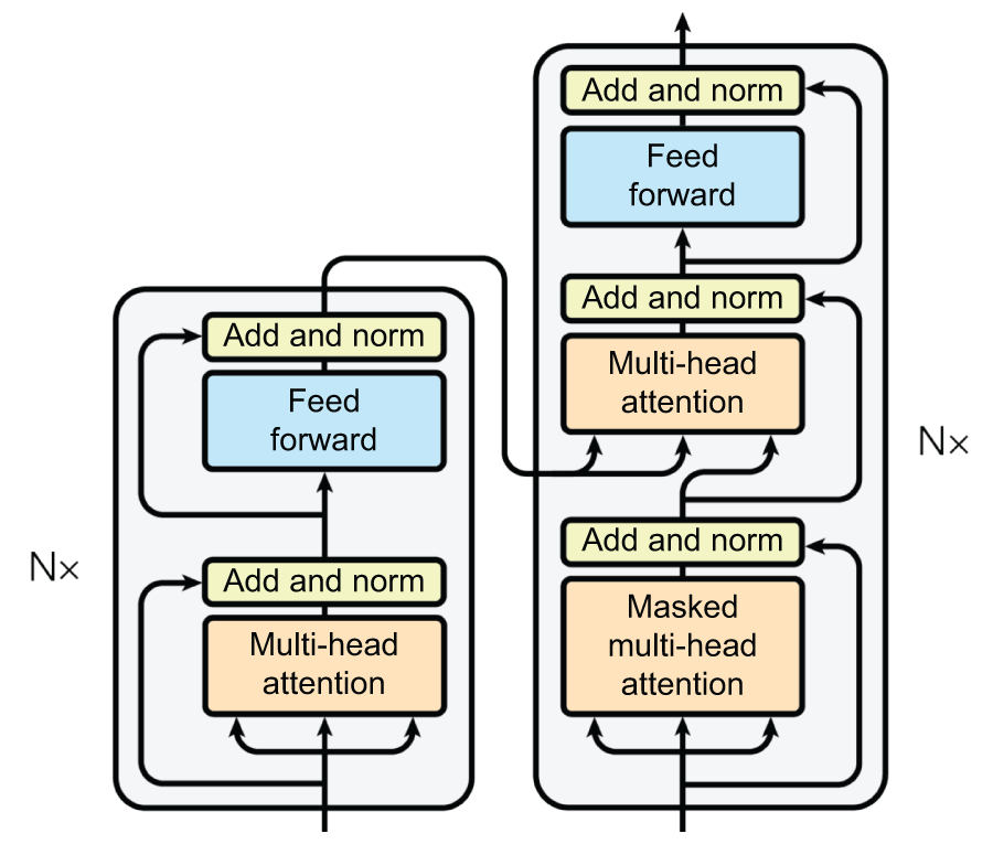
TransformerEncoder and TransformerDecoder blocks
Sequence-to-sequence learning with a Transformer
Let’s try putting this all together. We will use the same basic setup as our RNN
model, replacing the GRU layers with our TransformerEncoder and
TransformerDecoder. We will use 256 as the embedding size throughout the model,
except in the feedforward block. In the feedforward
block, we scale up the embedding size to 2048 before nonlinearity and scale back
to the model’s hidden size afterward. This large intermediate dimension works
well in practice.
hidden_dim = 256
intermediate_dim = 2048
num_heads = 8

source = keras.Input(shape=(None,), dtype="int32", name="english")
x = layers.Embedding(vocab_size, hidden_dim)(source)
encoder_output = TransformerEncoder(hidden_dim, intermediate_dim, num_heads)(
    source=x,
    source_mask=source != 0,
)

target = keras.Input(shape=(None,), dtype="int32", name="spanish")
x = layers.Embedding(vocab_size, hidden_dim)(target)
x = TransformerDecoder(hidden_dim, intermediate_dim, num_heads)(
    target=x,
    source=encoder_output,
    source_mask=source != 0,
)
x = layers.Dropout(0.5)(x)
target_predictions = layers.Dense(vocab_size, activation="softmax")(x)
transformer = keras.Model([source, target], target_predictions)
Let’s take a look at the summary of our Transformer model:
>>> transformer.summary()Model: "functional_3" ┏━━━━━━━━━━━━━━━━━━━━━━━┳━━━━━━━━━━━━━━━━━━━┳━━━━━━━━━━━━━┳━━━━━━━━━━━━━━━━━━━━┓ ┃ Layer (type) ┃ Output Shape ┃ Param # ┃ Connected to ┃ ┡━━━━━━━━━━━━━━━━━━━━━━━╇━━━━━━━━━━━━━━━━━━━╇━━━━━━━━━━━━━╇━━━━━━━━━━━━━━━━━━━━┩ │ english (InputLayer) │ (None, None) │ 0 │ - │ ├───────────────────────┼───────────────────┼─────────────┼────────────────────┤ │ embedding_5 │ (None, None, 256) │ 3,840,000 │ english[0][0] │ │ (Embedding) │ │ │ │ ├───────────────────────┼───────────────────┼─────────────┼────────────────────┤ │ not_equal_4 │ (None, None) │ 0 │ english[0][0] │ │ (NotEqual) │ │ │ │ ├───────────────────────┼───────────────────┼─────────────┼────────────────────┤ │ spanish (InputLayer) │ (None, None) │ 0 │ - │ ├───────────────────────┼───────────────────┼─────────────┼────────────────────┤ │ transformer_encoder_1 │ (None, None, 256) │ 1,315,072 │ embedding_5[0][0], │ │ (TransformerEncoder) │ │ │ not_equal_4[0][0] │ ├───────────────────────┼───────────────────┼─────────────┼────────────────────┤ │ not_equal_5 │ (None, None) │ 0 │ english[0][0] │ │ (NotEqual) │ │ │ │ ├───────────────────────┼───────────────────┼─────────────┼────────────────────┤ │ embedding_6 │ (None, None, 256) │ 3,840,000 │ spanish[0][0] │ │ (Embedding) │ │ │ │ ├───────────────────────┼───────────────────┼─────────────┼────────────────────┤ │ transformer_decoder_1 │ (None, None, 256) │ 1,578,752 │ transformer_encod… │ │ (TransformerDecoder) │ │ │ not_equal_5[0][0], │ │ │ │ │ embedding_6[0][0] │ ├───────────────────────┼───────────────────┼─────────────┼────────────────────┤ │ dropout_9 (Dropout) │ (None, None, 256) │ 0 │ transformer_decod… │ ├───────────────────────┼───────────────────┼─────────────┼────────────────────┤ │ dense_11 (Dense) │ (None, None, │ 3,855,000 │ dropout_9[0][0] │ │ │ 15000) │ │ │ └───────────────────────┴───────────────────┴─────────────┴────────────────────┘ Total params: 14,428,824 (55.04 MB) Trainable params: 14,428,824 (55.04 MB) Non-trainable params: 0 (0.00 B)
Our model has almost exactly the same structure as the GRU translation model we
trained earlier, with attention now substituting for recurrent layers as the
mechanism to pass information across the sequence. Let’s try training the model:
transformer.compile(
    optimizer="adam",
    loss="sparse_categorical_crossentropy",
    weighted_metrics=["accuracy"],
)
transformer.fit(train_ds, epochs=15, validation_data=val_ds)
After training, we get to about 58% accuracy: on average, the model correctly predicts the next word in the Spanish sentence 58% of the time. Something is off here. Training is worse than the RNN model by 7 percentage points. Either this Transformer architecture is not what it was hyped up to be, or we missed something in our implementation. Can you spot what it is?
This section is ostensibly about sequence models. In the previous chapter, we saw how vital word order could be to meaning. And yet, the Transformer we just built wasn’t a sequence model at all. Did you notice? It’s composed of dense layers that process sequence tokens independently of each other and an attention layer that looks at the tokens as a set. You could change the order of the tokens in a sequence, and you’d get identical pairwise attention scores and the same context-aware representations. If you were to rearrange every word in every English source sentence completely, the model wouldn’t notice, and you’d still get the same accuracy. Attention is a set-processing mechanism, focused on the relationships between pairs of sequence elements — it’s blind to whether these elements occur at the beginning, at the end, or in the middle of a sequence. So why do we say that Transformer is a sequence model? And how could it possibly be suitable for machine translation if it doesn’t look at word order?
For RNNs, we relied on the layer’s computation to be order aware. In the case of the Transformer, we instead inject positional information directly into our embedded sequence itself. This is called a positional embedding. Let’s take a look.
Embedding positional information
The idea behind a positional embedding is very simple: to give the model access to word order information, we will add the word’s position in the sentence to each word embedding. Our input word embeddings will have two components: the usual word vector, which represents the word independently of any specific context, and a position vector, which represents the position of the word in the current sentence. Hopefully, the model will then figure out how to best use this additional information.
The most straightforward scheme to add position information would be
concatenating each word’s position to its embedding vector. You’d add a
“position” axis to the vector and fill it with 0 for the first word in the
sequence, 1 for the second, and so on.
However, that may not be ideal because the positions can potentially be very large integers, which will disrupt the range of values in the embedding vector. As you know, neural networks don’t like very large input values or discrete input distributions.
The “Attention is all you need” authors used an interesting trick to encode word
positions: they added to the word embeddings a vector containing values in the
range [-1, 1] that varied cyclically depending on the position (they used cosine
functions to achieve this). This trick offers a way to uniquely characterize any
integer in a large range via a vector of small values. It’s clever, but it turns
out we can do something simpler and more effective: we’ll learn positional
embedding vectors the same way we learn to embed word indices. We’ll then
add our positional embeddings to the corresponding word embeddings to
obtain a position-aware word embedding. This is called a positional
embedding. Let’s implement it.
from keras import ops

class PositionalEmbedding(keras.Layer):
    def __init__(self, sequence_length, input_dim, output_dim):
        super().__init__()
        self.token_embeddings = layers.Embedding(input_dim, output_dim)
        self.position_embeddings = layers.Embedding(sequence_length, output_dim)

    def call(self, inputs):
        # Computes incrementing positions [0, 1, 2...] for each
        # sequence in the batch
        positions = ops.cumsum(ops.ones_like(inputs), axis=-1) - 1
        embedded_tokens = self.token_embeddings(inputs)
        embedded_positions = self.position_embeddings(positions)
        return embedded_tokens + embedded_positions
We would use this PositionalEmbedding layer just like a regular Embedding layer.
Let’s see it in action as we try training our Transformer for a second time.
hidden_dim = 256
intermediate_dim = 2056
num_heads = 8

source = keras.Input(shape=(None,), dtype="int32", name="english")
x = PositionalEmbedding(sequence_length, vocab_size, hidden_dim)(source)
encoder_output = TransformerEncoder(hidden_dim, intermediate_dim, num_heads)(
    source=x,
    source_mask=source != 0,
)

target = keras.Input(shape=(None,), dtype="int32", name="spanish")
x = PositionalEmbedding(sequence_length, vocab_size, hidden_dim)(target)
x = TransformerDecoder(hidden_dim, intermediate_dim, num_heads)(
    target=x,
    source=encoder_output,
    source_mask=source != 0,
)
x = layers.Dropout(0.5)(x)
target_predictions = layers.Dense(vocab_size, activation="softmax")(x)
transformer = keras.Model([source, target], target_predictions)
With the positional embedding now added to our model, let’s try training again:
transformer.compile(
    optimizer="adam",
    loss="sparse_categorical_crossentropy",
    weighted_metrics=["accuracy"],
)
transformer.fit(train_ds, epochs=30, validation_data=val_ds)
With positional information back in the model, things went much better. We
achieved a 67% accuracy when guessing the next word. It’s a noticeable
improvement from the GRU model, and that’s all the more impressive when you
consider that this model has half the parameters of the GRU counterpart.
There’s one other important thing to notice about this training run. Training is
noticeably faster than the RNN — each epoch takes about a third of the time.
This would be true even if we matched parameter count with the RNN model, and it
is a side effect of getting rid of the looped state passing of our GRU layers.
With attention, there is no looping computation to handle during training,
meaning that on a GPU or TPU, we can handle the entire attention computation in
one go. This makes the Transformer quicker to train on accelerators.
Let’s rerun generation with our newly trained Transformer. We can use the same
code as we did for our RNN sampling.
import numpy as np

spa_vocab = spanish_tokenizer.get_vocabulary()
spa_index_lookup = dict(zip(range(len(spa_vocab)), spa_vocab))

def generate_translation(input_sentence):
    tokenized_input_sentence = english_tokenizer([input_sentence])
    decoded_sentence = "[start]"
    for i in range(sequence_length):
        tokenized_target_sentence = spanish_tokenizer([decoded_sentence])
        tokenized_target_sentence = tokenized_target_sentence[:, :-1]
        inputs = [tokenized_input_sentence, tokenized_target_sentence]
        next_token_predictions = transformer.predict(inputs, verbose=0)
        sampled_token_index = np.argmax(next_token_predictions[0, i, :])
        sampled_token = spa_index_lookup[sampled_token_index]
        decoded_sentence += " " + sampled_token
        if sampled_token == "[end]":
            break
    return decoded_sentence

test_eng_texts = [pair[0] for pair in test_pairs]
for _ in range(5):
    input_sentence = random.choice(test_eng_texts)
    print("-")
    print(input_sentence)
    print(generate_translation(input_sentence))
Running the generation code, we get the following output:
-
The resemblance between these two men is uncanny.
[start] el parecido entre estos cantantes de dos hombres son asombrosa [end]
-
I'll see you at the library tomorrow.
[start] te veré en la biblioteca mañana [end]
-
Do you know how to ride a bicycle?
[start] sabes montar en bici [end]
-
Tom didn't want to do their dirty work.
[start] tom no quería hacer su trabajo [end]
-
Is he back already?
[start] ya ha vuelto [end]
Subjectively, the Transformer performs significantly better than the GRU-based translation model. It’s still a toy model, but it’s a better toy model.
The Transformer is a powerful architecture that has laid the basis for an explosion of interest in text-processing models. It’s also fairly complex, as deep learning models go. After seeing all of these implementation details, one might reasonably protest that this all seems quite arbitrary. There are so many small details to take on faith. How could we possibly know this choice and configuration of layers is optimal?
The answer is simple — it’s not. Over the years, a number of improvements have been proposed to the Transformer architecture by making changes to attention, normalization, and positional embeddings. Many new models in research today are replacing attention altogether with something less computationally complex as sequence lengths get very long. Eventually, perhaps by the time you are reading this book, something will have supplanted the Transformer as the dominant architecture used for language modeling.
There’s a lot we can learn from the Transformer that will stand the test of time. At the end of this chapter, we will discuss what makes the Transformer so effective. But it’s worth remembering that, as a whole, the field of machine learning moves empirically. Attention grew out of an attempt to augment RNNs, and after years of guessing and checking by a ton of people, it gave rise to the Transformer. There is little reason to think this process is done playing out.
Classification with a pretrained Transformer
After “Attention is all you need,” people started to notice how far Transformer training could scale, especially compared to models that had come before. As we just mentioned, one big plus was that the model is faster to train than RNNs. No more loops during training, which is always good when working with a GPU or TPU.
It is also a very data hungry model architecture. We actually got a little taste of this in the last section. While our RNN translation model plateaued in validation performance after 5 or so epochs, the Transformer model was still improving its validation score after 30 epochs of training.
These observations prompted many to try scaling up the Transformer with more data, layers, and parameters — with great results. This caused a distinctive shift in the field toward large pretrained models that can cost millions to train but perform noticeably better on a wide range of problems in the text domain.
For our last code example in the text section, we will revisit our IMDb text-classification problem, this time with a pretrained Transformer model.
Pretraining a Transformer encoder
One of the first pretrained Transformers to become popular in NLP was called BERT, short for Bidirectional Encoder Representations from Transformers[2]. The paper and model were released a year after “Attention Is All You Need.” The model structure was exactly the same as the encoder part of the translation Transformer we just built. This encoder model is bidirectional in that every position in the sequence can attend to positions in front of and behind it. This means it’s a good model for computing a rich representation of input text, but not a model meant to run generation in a loop.
BERT was trained in sizes between 100 million and 300 million parameters, much
bigger than the 14 million parameter Transformer we just trained. This meant the
model needed a lot of training data to perform well. To achieve this, the
authors used a riff on the classic language modeling setup called masked
language modeling. To pretrain the model, we take a sequence of text and
replace about 15% of the tokens with a special [MASK] token. The model will
attempt to predict the original masked token values during training. While the
classic language model, sometimes called a causal language model, attempts to
predict p(token|past tokens), the masked language model attempts to predict
p(token|surrounding tokens).
This training setup is unsupervised. You don’t need any labels about the text you feed in; for any text sequence, you can easily choose some random tokens and mask them out. That made it easy for the authors to find a large amount of text data needed to train models of this size. For the most part, they pulled from Wikipedia as a source.
Using pretrained word embeddings was already common practice when BERT was released — we saw this ourselves in the last chapter. But pretraining an entire Transformer gave something much more powerful — the ability to compute a word embedding for a word in the context of the words around it. And the Transformer allowed doing this at a scale and quality that were unheard of at the time.
The authors of BERT took this model, pretrained on a huge amount of text, and specialized it to achieve state-of-the-art results on several NLP benchmarks at the time. This marked a distinctive shift in the field toward using very large, pretrained models, often with only a small amount of fine-tuning. Let’s try this out.
Loading a pretrained Transformer
Instead of using BERT here, let’s use a follow-up model called RoBERTa[3], short for Robustly Optimized BERT. RoBERTa made some minor simplifications to BERT’s architecture, but most notably used more training data to improve performance. BERT used 16 GB of English language text, mainly from Wikipedia. The RoBERTa authors used 160 GB of text from all over the web. It’s estimated that RoBERTa cost a few hundred thousand dollars to train at the time. Because of this extra training data, the model performs noticeably better for an equivalent overall parameter count.
To use a pretrained model we will need a few things:
- A matching tokenizer — Used with the pretrained model itself. Any text must be tokenized in the same way as during pretraining. If the words of our IMDb reviews map to different token indices than they would have during pretraining, we cannot use the learned representations of each token in the model.
- A matching model architecture — To use the pretrained model, we need to recreate the math used internally by the model for pretraining exactly.
- The pretrained weights — These weights were created by training the model for about a day on 1,024 GPUs and billions of input words.
Recreating the tokenizer and architecture code ourselves would not be too hard.
The model internals almost exactly match the TransformerEncoder we built
previously. However, matching a model implementation is a time-consuming process, and
as we have done earlier in this book, we can instead use the KerasHub
library to access pretrained model implementations for Keras.
Let’s use KerasHub to load a RoBERTa tokenizer and model. We can use the
special constructor from_preset() to load a pretrained model’s
weights, configuration, and tokenizer assets from disk. We will load
RoBERTa’s base model, which is the smallest of the few pretrained checkpoints
released with the RoBERTa paper.
import keras_hub

tokenizer = keras_hub.models.Tokenizer.from_preset("roberta_base_en")
backbone = keras_hub.models.Backbone.from_preset("roberta_base_en")
The Tokenizer maps from text to sequences of integers, as we would
expect. Remember the SubWordTokenizer we built in the last chapter? RoBERTa’s
tokenizer is almost the same as that tokenizer, with minor tweaks to handle
Unicode characters from any language.
Given the size of RoBERTa’s pretraining dataset, subword tokenization is a
must. Using a character-level tokenizer would make input sequences way too long,
making the model much more expensive to train. Using a word-level tokenizer
would require a massive vocabulary to attempt to cover all the distinct words in
the millions of documents of text used from across the web. Getting good
coverage of words would blow up our vocabulary size and make the Embedding
layer at the front of the Transformer unworkably large. Using a subword
tokenizer allows the model to handle any word with only a 50,000-term vocabulary:
>>> tokenizer("The quick brown fox")Array([ 133, 2119, 6219, 23602], dtype=int32)
What is this Backbone we just loaded?
We saw in chapter 8 that a backbone is a term often used in computer vision for a network that maps from
input images to a latent space — basically a vision model without a head for
making predictions. In KerasHub, a backbone refers to any pretrained model that
is not yet specialized for a task. The model we just loaded takes in an input
sequence and embeds it to an output sequence with shape (batch_size,
sequence_length, 768), but it’s not set up for a particular loss function. You
could use it for any number of downstream tasks — classifying sentences,
identifying text spans with certain information, identifying parts of speech,
etc.
Next, we will attach a classification head to this backbone that specializes it for our IMDb review classification fine-tuning. You can think of this as attaching different heads to a screwdriver: a Phillips head for one task, a flat head for another.
Let’s take a look at our backbone. We loaded the smallest variant of RoBERTa here, but it still has 124 million parameters, which is the biggest model we have used in this book:
>>> backbone.summary()Model: "roberta_backbone" ┏━━━━━━━━━━━━━━━━━━━━━━━┳━━━━━━━━━━━━━━━━━━━┳━━━━━━━━━━━━━┳━━━━━━━━━━━━━━━━━━━━┓ ┃ Layer (type) ┃ Output Shape ┃ Param # ┃ Connected to ┃ ┡━━━━━━━━━━━━━━━━━━━━━━━╇━━━━━━━━━━━━━━━━━━━╇━━━━━━━━━━━━━╇━━━━━━━━━━━━━━━━━━━━┩ │ token_ids │ (None, None) │ 0 │ - │ │ (InputLayer) │ │ │ │ ├───────────────────────┼───────────────────┼─────────────┼────────────────────┤ │ embeddings │ (None, None, 768) │ 38,996,736 │ token_ids[0][0] │ │ (TokenAndPositionEmb… │ │ │ │ ├───────────────────────┼───────────────────┼─────────────┼────────────────────┤ │ embeddings_layer_norm │ (None, None, 768) │ 1,536 │ embeddings[0][0] │ │ (LayerNormalization) │ │ │ │ ├───────────────────────┼───────────────────┼─────────────┼────────────────────┤ │ embeddings_dropout │ (None, None, 768) │ 0 │ embeddings_layer_… │ │ (Dropout) │ │ │ │ ├───────────────────────┼───────────────────┼─────────────┼────────────────────┤ │ padding_mask │ (None, None) │ 0 │ - │ │ (InputLayer) │ │ │ │ ├───────────────────────┼───────────────────┼─────────────┼────────────────────┤ │ transformer_layer_0 │ (None, None, 768) │ 7,087,872 │ embeddings_dropou… │ │ (TransformerEncoder) │ │ │ padding_mask[0][0] │ ├───────────────────────┼───────────────────┼─────────────┼────────────────────┤ │ transformer_layer_1 │ (None, None, 768) │ 7,087,872 │ transformer_layer… │ │ (TransformerEncoder) │ │ │ padding_mask[0][0] │ ├───────────────────────┼───────────────────┼─────────────┼────────────────────┤ │ ... │ ... │ ... │ ... │ ├───────────────────────┼───────────────────┼─────────────┼────────────────────┤ │ transformer_layer_11 │ (None, None, 768) │ 7,087,872 │ transformer_layer… │ │ (TransformerEncoder) │ │ │ padding_mask[0][0] │ └───────────────────────┴───────────────────┴─────────────┴────────────────────┘ Total params: 124,052,736 (473.22 MB) Trainable params: 124,052,736 (473.22 MB) Non-trainable params: 0 (0.00 B)
RoBERTa uses 12 Transformer encoder layers stacked on top of each other. That’s a big step up from our translation model!
Preprocessing IMDb movie reviews
We can reuse the IMDb loading code we used in chapter 14 unchanged. This
will download the movie review data to a train_dir and test_dir and split a
validation dataset into a val_dir:
from keras.utils import text_dataset_from_directory

batch_size = 16
train_ds = text_dataset_from_directory(train_dir, batch_size=batch_size)
val_ds = text_dataset_from_directory(val_dir, batch_size=batch_size)
test_ds = text_dataset_from_directory(test_dir, batch_size=batch_size)
After loading, we once again have a training set of 20,000 movie reviews and a validation set of 5,000 movie reviews.
Before fine-tuning our classification model, we must tokenize our movie reviews
with the RoBERTa tokenizer we loaded. During pretraining, RoBERTa used a
specific form of “packing” tokens into a sequence, similar to what we did for
our translation model. Each sequence would begin with an <s> token, end with an
</s> token, and be followed by any number of <pad> tokens like this:
[
    ["<s>", "the", "quick", "brown", "fox", "jumped", ".", "</s>"],
    ["<s>", "the", "panda", "slept", ".", "</s>", "<pad>", "<pad>"],
]
It’s important to match the token ordering used for pretraining as closely as
possible; the model will train more quickly and accurately if we do. KerasHub
provides a layer for this type of token packing called the StartEndPacker. The
layer appends start, end, and padding tokens, trimming long sequences to a given
sequence length if necessary. Let’s use it along with our tokenizer.
def preprocess(text, label):
    packer = keras_hub.layers.StartEndPacker(
        sequence_length=512,
        start_value=tokenizer.start_token_id,
        end_value=tokenizer.end_token_id,
        pad_value=tokenizer.pad_token_id,
        return_padding_mask=True,
    )
    token_ids, padding_mask = packer(tokenizer(text))
    return {"token_ids": token_ids, "padding_mask": padding_mask}, label

preprocessed_train_ds = train_ds.map(preprocess)
preprocessed_val_ds = val_ds.map(preprocess)
preprocessed_test_ds = test_ds.map(preprocess)
Let’s take a look at a single preprocessed batch:
>>> next(iter(preprocessed_train_ds))({"token_ids": <tf.Tensor: shape=(16, 512), dtype=int32, numpy= array([[ 0, 713, 56, ..., 1, 1, 1], [ 0, 1121, 5, ..., 101, 24, 2], [ 0, 713, 1569, ..., 1, 1, 1], ..., [ 0, 100, 3996, ..., 1, 1, 1], [ 0, 100, 64, ..., 4655, 101, 2], [ 0, 734, 8, ..., 1, 1, 1]], dtype=int32)>, "padding_mask": <tf.Tensor: shape=(16, 512), dtype=bool, numpy= array([[ True, True, True, ..., False, False, False], [ True, True, True, ..., True, True, True], [ True, True, True, ..., False, False, False], ..., [ True, True, True, ..., False, False, False], [ True, True, True, ..., True, True, True], [ True, True, True, ..., False, False, False]])>}, <tf.Tensor: shape=(16,), dtype=int32, numpy=array([0, 1, ...], dtype=int32)>)
With our inputs preprocessed, we are ready to start fine-tuning our model.
Fine-tuning a pretrained Transformer
Before we fine-tune our backbone to predict movie reviews, we need to update it
so it outputs a binary classification label. The backbone outputs an entire
sequence with shape (batch_size, sequence_length, 768), where each
768-dimensional vector represents an input word in the context of its
surrounding words. Before predicting a label, we must condense this sequence to
a single vector per sample.
One option would be to do mean pooling or max pooling across the whole sequence, computing an average of all token vectors. What works slightly better is simply using the first token’s representation as the pooled value. This is due to the nature of the attention in our model — the first position in the final encoder layer will be able to attend to all other positions in the sequence and pull information from them. So rather than pooling information with something coarse, like taking an average, attention allows us to pool information contextually across the sequence.
Let’s now add a classification head to our backbone. We will also add one final
Dense projection with a nonlinearity before generating an output prediction.
inputs = backbone.input
x = backbone(inputs)
# Uses the hidden representation of the first token
x = x[:, 0, :]
x = layers.Dropout(0.1)(x)
x = layers.Dense(768, activation="relu")(x)
x = layers.Dropout(0.1)(x)
outputs = layers.Dense(1, activation="sigmoid")(x)
classifier = keras.Model(inputs, outputs)
With that, we are ready to fine-tune and evaluate the model on the IMDb dataset.
classifier.compile(
    optimizer=keras.optimizers.Adam(5e-5),
    loss="binary_crossentropy",
    metrics=["accuracy"],
)
classifier.fit(
    preprocessed_train_ds,
    validation_data=preprocessed_val_ds,
)
Finally, let’s evaluate the trained model:
>>> classifier.evaluate(preprocessed_test_ds)[0.168127179145813, 0.9366399645805359]
In just a single epoch of training, our model reached 93%, a noticeable improvement from the 90% ceiling we hit in our last chapter. Of course, this is a far more expensive model to use than the simple bigram classifier we built previously, but there are clear benefits to using such a large model. And this is all with the smaller size of the RoBERTa model. Using the larger 300 million parameter model, we could achieve an accuracy of over 95%.
What makes the Transformer effective?
In 2013, at Google, Tomas Mikolov and his colleagues noticed something remarkable. They were building a pretrained embedding called “Word2Vec,” similar to the Continuous Bag of Words (CBOW) embedding we built in the last chapter. Much like our CBOW model, their training objective sought to turn correlation relationships between words into distance relationships in the embedding space: a vector was associated with each word in a vocabulary, and the vectors were optimized so that the dot-product (cosine proximity) between vectors representing frequently co-occurring words would be closer to 1, while the dot-product between vectors representing rarely co-occurring words would be closer to 0.
They found that the resulting embedding space did much more than capture
semantic similarity. It featured some form of emergent learning — a sort of
“word arithmetic.” A vector existed in the space that you could add to many male
nouns to obtain a point that would land close to its female equivalent, as in
V(king) - V(man) + V(woman) = V(queen), a gender vector. This was quite
surprising; the model had not been trained for this in any explicit way. There
seemed to be dozens of such magic vectors — a plural vector, a vector to go
from wild animals’ names to their closest pet equivalent, etc.
Fast-forward about 10 years — we are now in the age of large, pretrained Transformer models. On the surface, these models couldn’t seem any further from the primitive Word2Vec model. A Transformer can generate perfectly fluent language — a feat Word2Vec was entirely incapable of. As we will see in the next chapter, such models can seem knowledgeable about virtually any topic. And yet, they actually have a lot in common with good old Word2Vec.
Both models seek to embed tokens (words or subwords) in a vector space. Both rely on the same fundamental principle to learn this space: tokens that appear together end up close in the embedding space. The distance function used to compare tokens is cosine distance in both cases. Even the dimensionality of the embedding space is similar: a vector with somewhere between 1,000 and 10,000 dimensions to represent each word.
At this point, you might interject: A Transformer is trained to predict missing words in a sequence, not to group tokens in an embedding space. How does the language model loss function relate to Word2Vec’s objective of maximizing the dot-product between co-occurring tokens? The answer is the attention mechanism.
Attention is, by far, the most critical component in the Transformer architecture. It’s a mechanism for learning a new token embedding space by linearly recombining token embeddings from some prior space, in weighted combinations that give greater importance to tokens that are already “closer” to each other (i.e., that have a higher dot-product). It will tend to pull together the vectors of already close tokens, resulting over time in a space where token correlation relationships turn into embedding proximity relationships (in terms of cosine distance). Transformers work by learning a series of incrementally refined embedding spaces, each based on recombining elements from the previous one.
Attention provides Transformers with two crucial properties:
- The embedding spaces they learn are semantically continuous — that is, moving a bit in an embedding space only changes the human-facing meaning of the corresponding tokens by a bit. The Word2Vec space also exhibited this property.
- The embedding spaces they learn are semantically interpolative — that is, taking the intermediate point between two points in an embedding space produces a point representing the “intermediate meaning” between the corresponding tokens. This comes from the fact that each new embedding space is built by interpolating between vectors from the previous space.
This is not entirely unlike the way the brain learns. The key learning principle in the brain is Hebbian learning — in short, “neurons that fire together, wire together.” Correlation relationships between neural firing events (which may represent actions or perceptual inputs) are turned into proximity relationships in the brain network, just like the Transformer and Word2Vec turn correlation relationships into vector proximity relationships. Both are maps of a space of information.
Of course, there are significant differences between Word2Vec and the Transformer. Word2Vec was not designed for generative text sampling. A Transformer can get far bigger and can encode vastly more complex transformations. The thing is, Word2Vec is very much a toy model: it is to today’s language models as a logistic regression on MNIST pixels is to state-of-the-art computer vision models. The fundamental principles are mostly the same, but the toy model lacks any meaningful representation power. Word2Vec wasn’t even a deep neural network — it had a shallow, single-layer architecture. Meanwhile, today’s Transformer models have the highest representation power of any model anyone has ever trained — they feature dozens of stacked attention and feedforward layers, and their parameter count ranges in the billions.
Like with Word2Vec, the Transformer learns useful semantic functions as a by-product of organizing tokens into a vector space. But thanks to this increased representation power and a much more refined autoregressive optimization objective, we’re no longer confined to linear transformations like a gender vector or a plural vector. Transformers can store arbitrarily complex vector functions — so complex, in fact, that it would be more accurate to refer to them as vector programs rather than functions.
Word2Vec enabled you to do basic things like plural(cat) → cats or
male_to_female(king) → queen. Meanwhile, a large Transformer model can do pure
magic — things like write_this_in_style_of_shakespeare("...your poem...") →
"...new poem...". And a single model can contain millions of such programs.
You can see a Transformer as analogous to a database: it stores information you can retrieve via the tokens you pass in. But there are two important differences between a Transformer and a database.
The first difference is that a Transformer is a continuous, interpolative kind of database. Instead of being stored as a set of discrete entries, your data is stored as a vector space — a curve. You can move around on the curve (it’s semantically continuous, as we discussed) to explore nearby, related points. And you can interpolate on the curve between different data points to find their in-between. This means that you can retrieve a lot more from your database than you put into it — although not all of it will be accurate or meaningful. Interpolation can lead to generalization, but it can also lead to hallucinations — a significant problem facing the generative language models trained today.
The second difference is that a Transformer doesn’t just contain data. For models like RoBERTa, trained on hundreds of thousands of documents scraped from the internet, there is a lot of data: facts, places, people, dates, things, and relationships. But it’s also — perhaps primarily — a database of programs.
They’re different from the kind of programs you’re used to dealing with, mind you. These are not like Python programs — series of symbolic statements processing data step by step. Instead, these vector programs are highly nonlinear functions that map the latent embedding space unto itself, analogous to Word2Vec’s magic vectors, but far more complex.
In the next chapter, we will push Transformer models to an entirely new scale. Models will use billions of parameters and train on trillions of words. Output from these models can often feel like magic — like an intelligent operator sitting inside our model and pulling the strings. But it’s important to remember that these models are fundamentally interpolative — thanks to attention, they learn an interpolative embedding space for a significant chunk of all text written in the English language. Wandering this embedding space can lead to interesting, unexpected generalizations, but it cannot synthesize something fundamentally new with anything close to genuine, human-level intelligence.
Summary
- A language model is a model that learns a specific probability
distribution —
p(token|past tokens):- Language models have broad applications, but the most important is that you can generate text by calling them in a loop, where the output token at one time step becomes the input token in the next.
- A masked language model learns a related probability distribution
p(tokens|surrounding tokens)and can be helpful for classifying text and individual tokens. - A sequence-to-sequence language model learns to predict the next token given both past tokens in a target sequence and an entirely separate, fixed source sequence. Sequence-to-sequence models are useful for problems like translation and question answering.
- A sequence-to-sequence model usually has two separate components. An encoder computes a representation of the source sequence, and a decoder takes this representation as input and predicts the next token in a target sequence based on past tokens.
- Attention is a mechanism that allows a model to pull information from
anywhere in a sequence selectively based on the context of the token
currently being processed:
- Attention avoids the problems RNNs have with long-range dependencies in text.
- Attention works by taking the dot-product of two vectors to compute an attention score. Vectors near each other in an embedding space will be summed together in the attention mechanism.
- The Transformer is a sequence modeling architecture that uses attention as
the only mechanism to pass information across a sequence:
- The Transformer works by stacking blocks of alternating attention and two-layer feedforward networks.
- The Transformer can scale to many parameters and lots of training data while still improving accuracy in the language modeling problem.
- Unlike RNNs, the Transformer involves no sequence-length loops at training time, making the model much easier to train in parallel across many machines.
- A Transformer encoder uses bidirectional attention to build a rich representation of a sequence.
- A Transformer decoder uses causal attention to predict the next word in a language model setup.